Simplicial Lattice and Lagrange Elements

We use Lagrange elements as an example to introduce the simplicial lattice and construction of finite elements based on a decomposition of the simplicial lattice. Brief explanation will be given after some slides. Proofs included in the slides are short and less rigorous. The readers are encouraged to read the reference for all details.

Reference: Geometric decompositions of the simplicial lattice and smooth finite elements in arbitrary dimension Long Chen and Xuehai Huang. arXiv. 2021.

To leave comments (in math), please visit my UCI blog

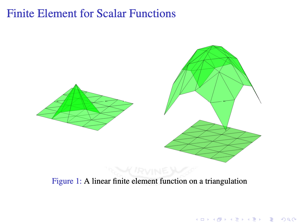
Finite Elements

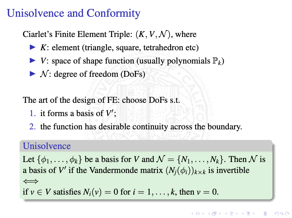
The DoFs are not just functional defined on the shape function $V$​. Indeed it is implicitly assumed a DoF $N(u)$​ can be extended to function $u$​ in a larger space $U$​ so that $V\subset U$​​.

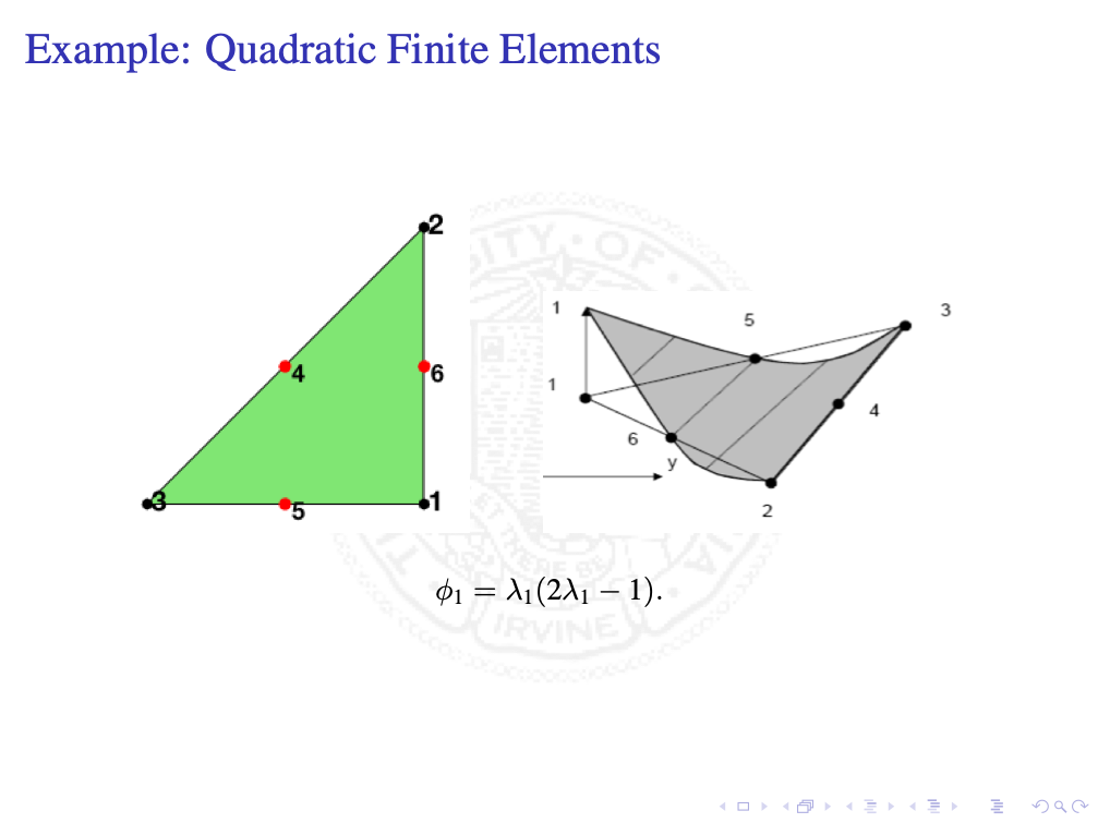
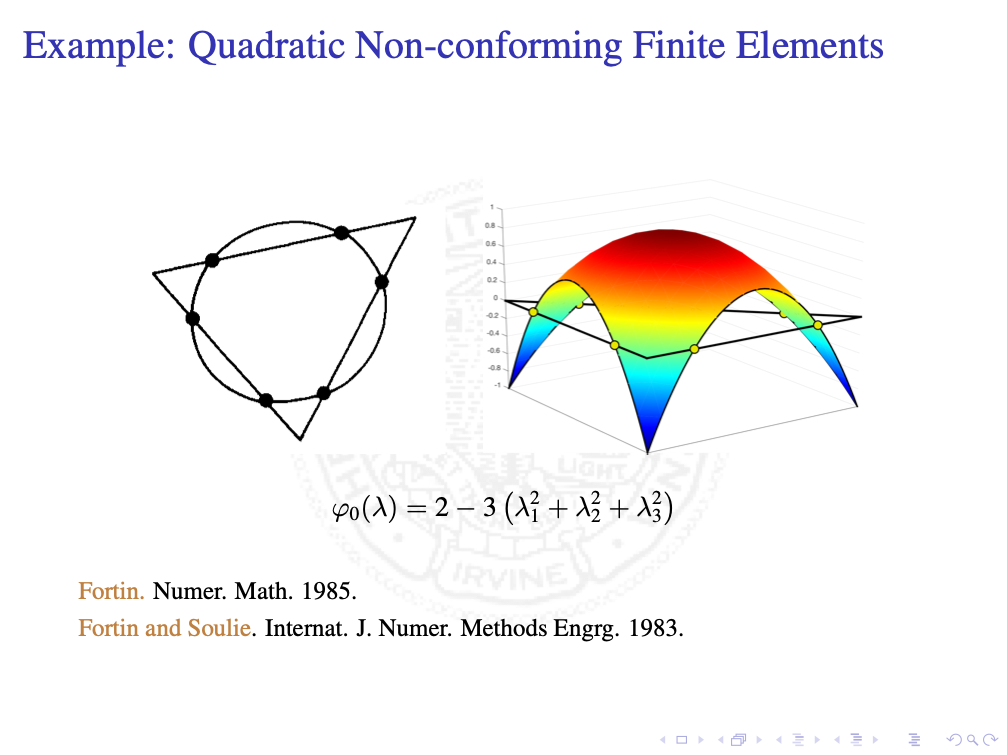
Let’s look at two examples. The shape function is now the quadratic polynomial whose dimension is $6$​​​. Function values at $3$​​ vertices and middle points of $3$​​ edges are well defined DoFs. But $6$​ points sitting on the same circle are not as a qudratic polynomial can vanish at those $6$​​ points only. This is the example found by Fortin when he wants to generalize the linear CR non-conforming element to quadratic.

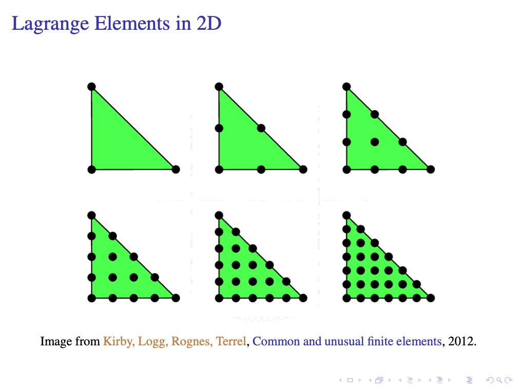
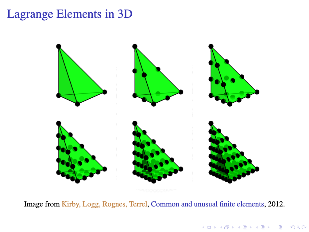
DoFs for Lagrange elements on triangules and tetrahedron are well knowns. One can use function values on the nodes listed below. Later on we shall give a unified proof on the uni-sovlence.

Simplex

Let $\boldsymbol x_{i}=(x_{1,i}, \cdots, x_{n,i})^{\intercal}, i=1,\cdots, n+1$ be $n+1$ points in $\mathbb R^n$. We say $\boldsymbol x_1, \cdots, \boldsymbol x_{n+1}$ do not all lie in one hyper-plane if the $n$-vectors $\boldsymbol x_1\boldsymbol x_{2},\cdots, \boldsymbol x_1\boldsymbol x_{n+1}$​ are independent. This is equivalent to the matrix:

\[A = \left ( \begin{array}{cccc} x_{1,1} & x_{1,2} & \ldots & x_{1,n+1} \\ x_{2,1} & x_{2,2} & \ldots & x_{2,n+1} \\ \vdots & \vdots & & \vdots \\ x_{n,1} & x_{n,2} & \ldots & x_{n,n+1}\\ 1 & 1 & \ldots & 1 \end{array} \right)\]

is non-singular. Given any point $\boldsymbol x=(x_1,\cdots, x_n)\in \mathbb R^n$, by solving the following linear system

\[A \left ( \begin{array}{c} \lambda_1\\ \vdots\\ \lambda_n\\ \lambda_{n+1} \end{array}\right ) = \left ( \begin{array}{c} x_1\\ \vdots\\ x_{n}\\ 1 \end{array}\right ), \tag{$\ast$} \label{eq:Alambda}\]

we obtain unique $n+1$ real numbers $\lambda_{i}(\boldsymbol x), 1\leq i\leq n+1$, such that for any $\boldsymbol x\in \mathbb R^n$ \(\boldsymbol x=\sum _{i=1}^{n+1}\lambda _i(\boldsymbol x)\boldsymbol x_i, \; \text{ with } \; \sum _{i=1}^{n+1}\lambda _i(\boldsymbol x)=1.\)

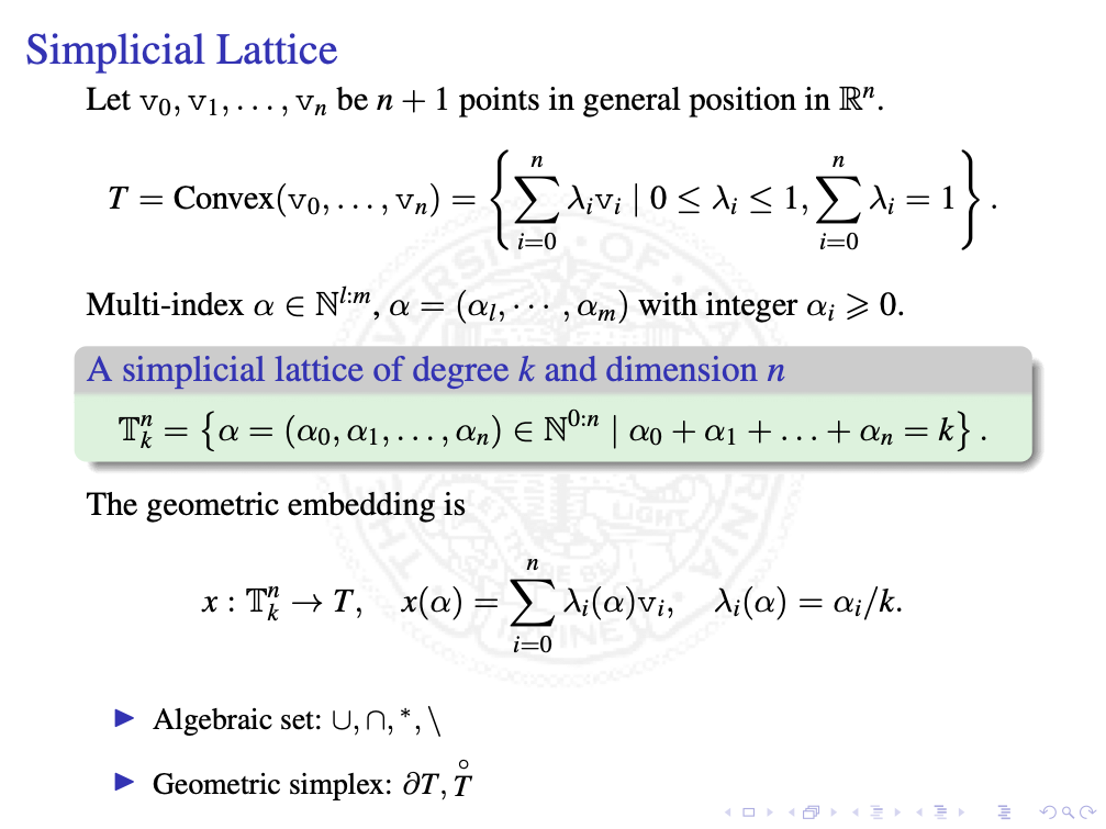
Given an integer $d\leq n$​, the convex hull of the $d+1$​ points $\boldsymbol x_1, \ldots, \boldsymbol x_{d+1}$​ in $\mathbb R^n$​ \(\tau :=\{\boldsymbol x=\sum _{i=1}^{d+1}\lambda _i\boldsymbol x_i \, | \, 0\leq \lambda_i\leq 1, i=1:d+1, \sum _{i=1}^{d+1}\lambda _i=1 \}\) is defined as a geometric $d$​​-simplex generated (or spanned) by the vertices $\boldsymbol x_1, \cdots, \boldsymbol x_{d+1}$​​. For example, a triangle is a $2$-simplex and a tetrahedron is a $3$​​-simplex.

The numbers $\lambda_1(\boldsymbol x),\ldots,\lambda_{d+1}(\boldsymbol x)$​​​ are called barycentric coordinates of $\boldsymbol x$​​​ with respect to the $d+1$​​​ vertices $\boldsymbol x_1, \ldots, \boldsymbol x_{d+1}$​​​ .

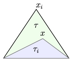
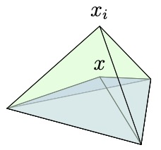
There is a simple geometric meaning of the barycentric coordinates. Given a $\boldsymbol x\in \tau$, let $\tau_i(\boldsymbol x)$ be the simplex with vertices $\boldsymbol x_i$ replaced by $\boldsymbol x$. Then, by the Cramer’s rule for solving \eqref{eq:Alambda}, \(\lambda _i(\boldsymbol x) = \frac{|\tau _i(\boldsymbol x)|}{|\tau|},\) where $|\cdot|$ is the Lebesgue measure in $\mathbb R^d$, namely area in two dimensions and volume in three dimensions. Note that $\lambda_i(\boldsymbol x)$ is an affine function of $\boldsymbol x$ and vanished on the face opposite to $\boldsymbol x_i$.

Simplicial Lattice

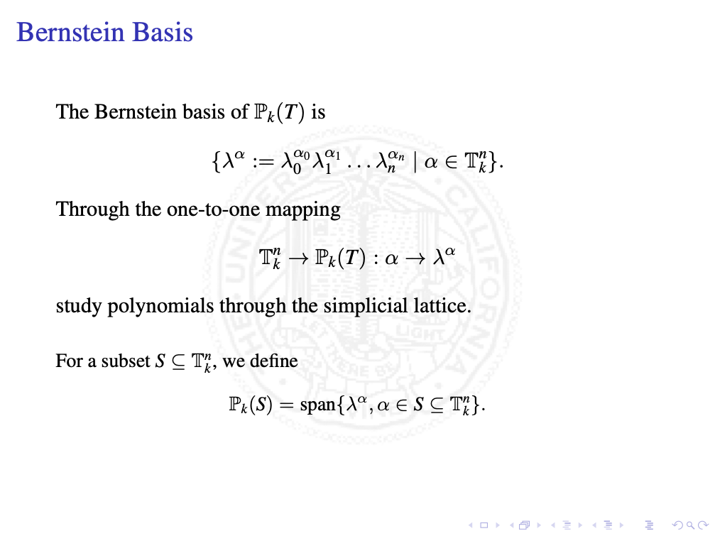
We will introduce an important concept: simplicial lattice for the unified construction of finite elements on simplex in general dimensions. Through the Berstein basis, it is one-to-one mapped to a polynomial and thus the study of $\mathbb P_k(T)$​ can be transfered to the simplicial lattice.

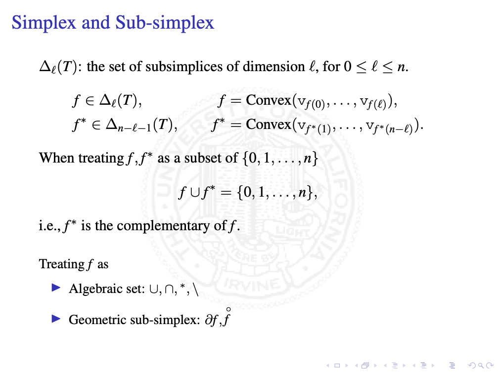
Sub-simplex and Bubble Functions

We need more notation on the sub-simplex. The following notation system is simplified from the reference

• D. N. Arnold, R. S. Falk, and R. Winther. Geometric decompositions and local bases for spaces of finite element differential forms. Computer Methods in Applied Mechanics and Engineering, 198(21-26):1660– 1672, 2009

The simplication is: we use one symbol $f$ for both the algebraic set and the geometric sub-simplex. Also since no differential form is involved, there is no ordering assumed in the set.

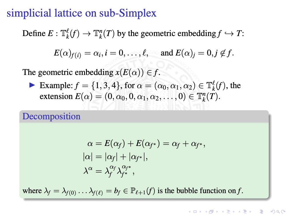
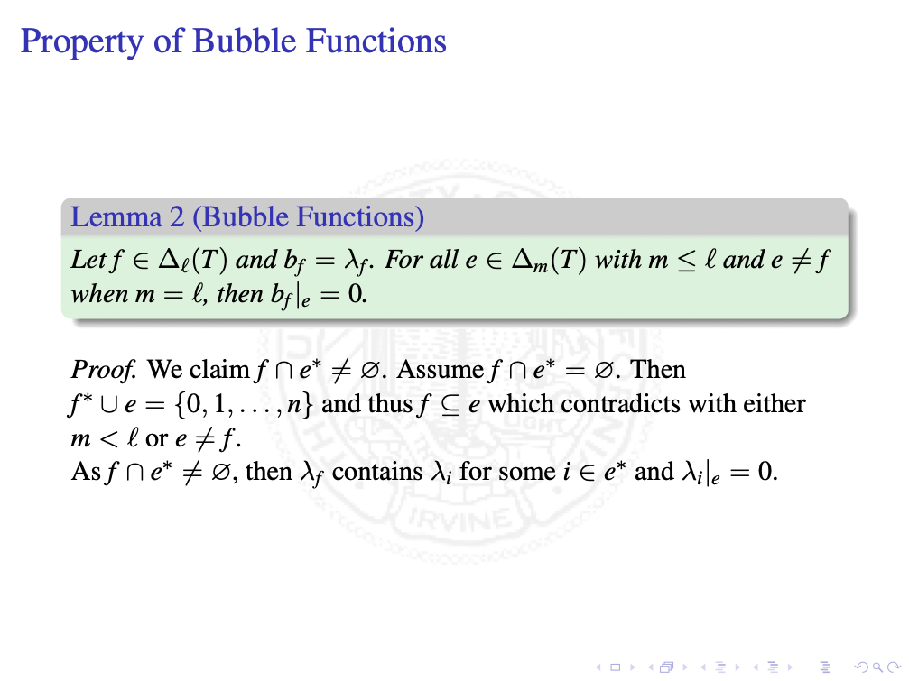
There is a nice property of the bubble function. The bubble function $b_f$​ on a face will vanish on all lower dimensional sub-simplex $e$​ no matter if $e\subset f$​ or not. It also vanish on other faces $f’$​ with the same dimension.

Lagrange Finite Elements

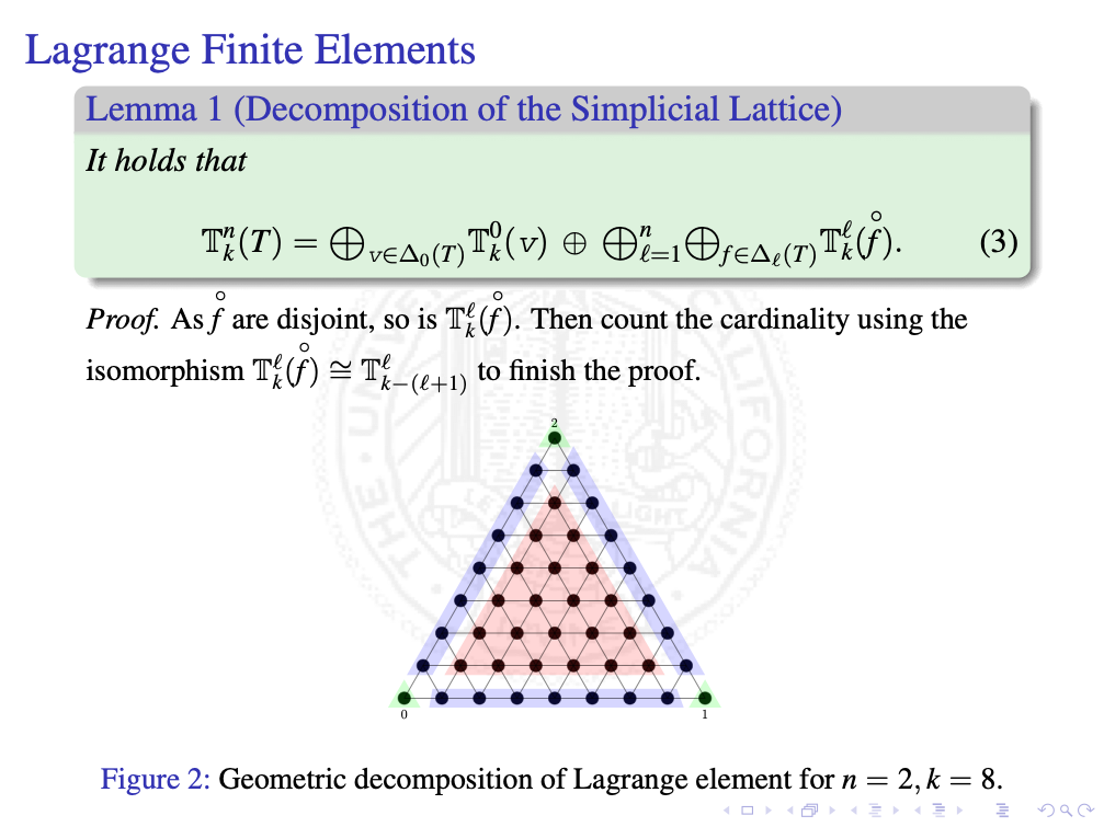
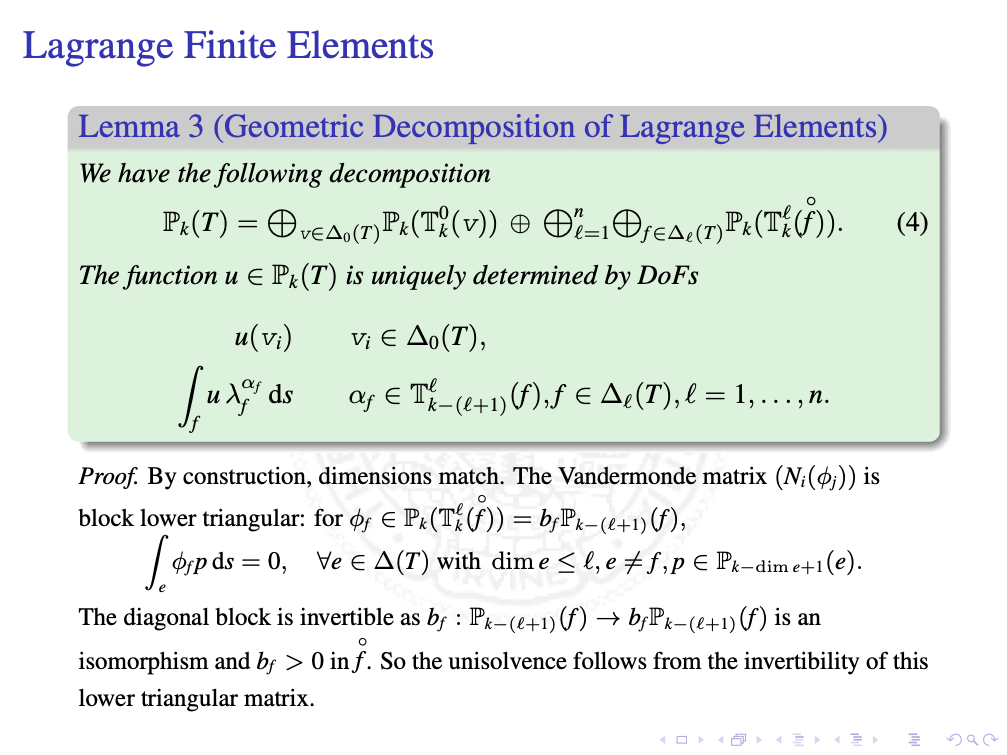
We can construct Lagrang finite elements based on a decomposition of the simplicial lattice. The DoFs are integrals on sub-simplex. Using the property of the bubble functions, the resulting DoF-Fun matrix is block lower triangular and the diagonal block is a Gram matrix $(\int_f b_f p_ip_j \, ds)$, which is symmetric and positive definite (SPD). If using function values, the matrix $( p_i(x_j))$ is still invertiable for the sub-simplex lattice which can be proved by recursion.

---

To leave comments, please register a GitHub account and then you can sign in GitHub to write comments using Markdown and LaTeX.