Introduction to Calculus of Variation

Problem Formulation

A typical problem in the calculus of variation is in the form \(\inf_{u\in \mathcal M} I(u), \tag{1}\label{eq:cov}\)

where the integral functional is

\[I(u) = \int_{\Omega} L(x, u(x), \nabla u(x))\, dx,\]

• $\Omega\subset \mathbb R^d$ is an open domain;
• $\mathcal M$ is a subset of some function spaces defined on $\Omega$;
• $L$ is called Lagrangian.

When considering 1-d problems, i.e., $d=1$, usually we write the independent variable as $t$, $\Omega = (a,b)$, and $L = L(t, x(t), \dot{x}(t))$.

So $\eqref{eq:cov}$ is a minimization problem or in general optimization problems (finding minimum, maximum, or saddle points) which shares a lot of similarities with the calculus problem \(\inf_{x\in M} f(x).\tag{2}\label{eq:opt}\)

It is highly recommended to use \eqref{eq:opt} to help understanding concepts and key points of \eqref{eq:cov}.

What is the main difference between the calculus problem $\eqref{eq:opt}$ and the calculus of variation problem $\eqref{eq:cov}$?

• The dependence in $\eqref{eq:opt}$ is two-layer $x \mapsto f(x)$;
• While $\eqref{eq:cov}$ contains three-layers: $x\mapsto u(x) \mapsto I(u)$;

The independent variable in $I(\cdot)$ is a function $u$ which itself is a function of $x$ in some Euclidean space $\mathbb R^d$. Function of functions is called functional. Therefore functional analysis is indispensable for Calculus of Variation.

The subset $\mathcal M$ in $\eqref{eq:cov}$ is in some function space, say $H^1(\Omega)$, while $M$ in $\eqref{eq:opt}$ is a subset in $\mathbb R^d$ which is finite dimensional. The function space is usually infinite dimensional and thus many results or properties of finite dimensional linear spaces should be re-examined in the infinite dimensional space. The fundamental difference is the compactness. In finite dimensional normed vector space, a set is compact if and only it is bounded and closed. Recall that the infimum of problem $\eqref{eq:opt}$ exists if $M$ compact. In infinite dimensional spaces, boundedness and closedness are necessary but not sufficient. Weaker topologies should be introduced to enable the unit ball is compact with respect to that topology.

Tools

We now summarize three fundamental tools used in Calculus of Variation.

• Chain rule of differentiation. (Easy but tedious)

• Integration by parts. (Medium especially in high dimensions)
• Change of variables. (Hard and deep)

When taking derivatives, we have to be careful on the dependence of variables. For example, when write the Lagrangian as $L(x, u, p)$, variables $(u,p)$ are independent. While in the notation $L(x, u(x), \nabla u(x))$, $p = \nabla u$ is substituted and therefore the 2nd and 3rd variables are now related.

The functional $I(\cdot)$ involves the derivative $\nabla u$ and integral $\int_{\Omega}$. The interplay of these two is integration by parts. When the domain $\Omega$ is less smooth (e.g. a polyhedron), integration by parts should be applied piecewisely and jump conditions on lower dimensional faces will appear.

Change of variables turns out to be the key tool which leads to the deepest results in calculus of variations. Examples include: Legendre transform and Noether’s theorem.

Legendre transform changes a Lagrangian to a Hamiltonian and the Euler-Lagrange equation into the Hamiltonian system. The further introduce of a scalar potential gives the Hamilton-Jacobi equation. Different variables and different equations reveal different structures for the same physical system.

If the functional is invariant under some transformations, then there is a conservation law. This is the most beautiful and the deepest result in calculus of variations: Noether’s theorem.

An Example

We end this introduction by an 1-D example. Recall that in 1-D, we use $t\in \mathbb R$ instead of $x$, and $\dot{x}$ instead of $\nabla u$. Note that although $t\in \mathbb R$, the function $x(t)$ could be a curve in space, i.e., $x$ could be a vector. Consider \(\inf_{x\in \mathcal M} \int_0^1 L (t, x(t), \dot{x}(t))\, d t,\)

with a typical example

• $\mathcal M = \{x\in C^1(0,1), x(0) = x_0, x(1) = v_1\}$

• $\displaystyle L(t,x,v) = \frac{1}{2}m |v|^2 - U(x)$ is the difference of kinetic energy $T(v) = \frac{1}{2}m |v|^2 $ and potential energy $U(x)$.

Recall that the first order condition for $\eqref{eq:opt}$ is $f’(x) = 0$. But now $x = x(t)$ itself is a function and may change in every point $t\in (0,1)$. How to take derivative of a function?

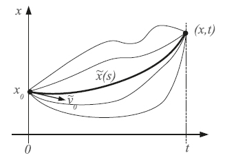
The idea is to introduce a variation of the function. Let $\phi$ be a test function in $\mathcal M_0$ satisfies certain boundary conditions so that $x+\epsilon \phi\in \mathcal M$. The term $\epsilon \phi$ is an variation of $x$. Define $f(\epsilon): = I(x+\epsilon \phi)$. Then $x$ is an infimum of $\eqref{eq:cov}$ if and only if $0$ is a minimum of $f(\epsilon)$. So the optimality condition of an extreme curve $x$ of $I(x)$ is characterized as

\[f'(0) = \frac{\text{d}}{\text{d} \epsilon} I(x+\epsilon \phi) \big|_{\epsilon = 0} = 0,\]

• Chain rule. By the chain rule, we obtain the variational form of Euler-Lagrange equation

\[\tag{3}\label{intro:weakEL} \int_0^1 L_x(t, x, \dot{x}) \phi + L_v(t, x, \dot{x}) \dot{\phi} = 0 \quad \forall \phi \in \mathcal M_0.\]

• Integration by parts. Take $\phi \in C^{\infty}_0(0,1) = {\phi \in C^{\infty}(0,1): \phi^{(\alpha)}(0)=\phi^{(\alpha)}(1) = 0, \forall \alpha \in \mathbb N}$ and apply integration by parts, we obtain

\[\int_0^1 \left [L_x(t, x, \dot{x}) - \frac{\text{d}}{\text{d} t} L_v(t, x, \dot{x})\right ] \phi = 0 \quad \forall \phi \in C^{\infty}_0(0,1)\subset \mathcal M_0.\]

The boundary terms disappeared as $\phi \in C^{\infty}_0(0,1)$. Now use $C^{\infty}_0(0,1)$ is dense in $L^2(0,1)$, we conclude the strong form of Euler-Lagrange equation

\[\tag{4}\label{intro:1dEL} - \frac{\text{d}}{\text{d} t} L_v(t, x(t), \dot{x}(t)) + L_x (t, x(t), \dot{x}(t)) = 0.\]

For $L(t,x,v) = \frac{1}{2}m |v|^2 - U( x)$, $\eqref{intro:1dEL}$ becomes the Newton’s equation

\[m \ddot{x} = F,\quad \text{ with }F = - \nabla_x U.\]

which is known as “Hamilton’s form of the principle of least action”.

• Change of variables. Consider change of variables

\[\left\{ \, \begin{aligned} q &= x, \\ p & = L_{v}(t, q,\dot{q}). \end{aligned}\right.\]

Assume $L$ is convex in $v$. Then we can solve $\dot{q} = \dot{q}(p,q,t)$. Define Hamiltonian

\[\tag{5}\label{intro:Hamiltonian} H(p,q,t) := p \dot{q}(p) - L(t, q, \dot{q}(p)).\]

Then the Euler-Lagrange becomes the Hamiltonian system

\[\tag{6}\label{eq:Hsystem} \left \{ \, \begin{aligned} \dot{p} &= - H_q,\\ \dot{q} &= H_p.\\ \end{aligned}\right.\]

To derive the Hamiltonian system, we apply total differentiation to both sides of $\eqref{intro:Hamiltonian}$ to get \(\text{d} H= H_p \text{d} p + H_q \text{d} q+ H_t \text{d} t\) and \(p \text{d} \dot{q}+\dot{q} \text{d} p-L_t \text{d} t - L_q \text{d} q- L_v \text{d} \dot{q} = \dot{q} \text{d} p- \dot{p} \text{d} q -L_t \text{d} t.\)

The last step is due to $p = L_v$ by definition and E-L equation $L_q = \dot{p}$ in terms of new variables.

When Hamiltonian $H(p,q)$ is independent of $t$, for solutions to the Hamiltonian system, we obtain the conservation of Hamiltonian, i.e.

\[\frac{\text{d} }{\text{d} t}H(p(t),q(t)) = H_p \dot{p} + H_q \dot{q} = 0.\]

An important example is $L = T - U$. For $T (v) = \frac{1}{2}m |v|^2$, the variable $p = mv$ is the momentum. Then

\[H = p\dot{q}(p) - L = pv - T(v) - U(q) = \frac{1}{2}m |v|^2 + U(q) = T + U\]

is the total energy. From Noether’s point of view, the conservation of energy is due to the translation invariant in time. Better using symmetry instead of invariance.

• Time translation symmetry: conservation of energy;

• Space translation symmetry: conservation of momentum;

• Rotation symmetry: conservation of angular momentum.

Even more deep double way connection is: a symmetry implies a conservation law, and the associated conserved quantity generates the symmetry. The later motivates lots of theoretical physics from experimental physics. First observe some conserved quantity in experiment first and then find the symmetry generated by this quantity.