Project: 1-D Finite Difference Method
The purpose of this project is to introduce the finite difference method for solving differential equations in 1-D. Consider 1-D Poisson equation in $(0,1)$ with Dirichlet boundary condition
\[- u'' = f \,\; {\rm in }\, (0,1), \quad u(0) = a, u(1) = b.\]Step 1: Generate a grid
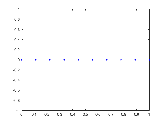
Generate a vector representing a uniform grid with size h of (0,1).
N = 10;
x = linspace(0,1,N);
plot(x,0,'b.','Markersize',16)
Step 2: Generate A Matrix Equation
Based on a grid, the function $u$ is discretized by a vector u. The
derivative $u’, u’’$ are approximated by centeral finite difference:
The equation $-u’‘(x) = f(x)$ is discretized at $x_i, i=1,…,N$ as
\[\frac{-u(i-1) + 2u(i) - u(i+1)}{h^2} \quad = f(i),\]where $f(i) = f(x_i)$. These linear equations can be written as a matrix
equation A*u = f, where A is a tri-diagonal matrix (-1,2,-1)/h^2.
n = 5;
e = ones(n,1);
A = spdiags([e -2*e e], -1:1, n, n);
display(full(A));
ans =

    -2     1     0     0     0
     1    -2     1     0     0
     0     1    -2     1     0
     0     0     1    -2     1
     0     0     0     1    -2
We use spdiags to speed up the generation of the matrix since the matrix is sparse. Compare diag and spdiags.
Stpe 3: Modify the Matrix Equation to Impose Boundary Conditions
The discretization fails at boundary vertices since no nodes outside the
interval. Howevery the boundary value is given by the problem: u(1) = a,
u(N) = b.
These two equations can be included in the matrix by changing A(1,:) =
[1, 0 ..., 0] and A(:,N) = [0, 0, ..., 1] and f(1) = a/h^2, f(N) =
b/h^2.
A(1,1) = 1;
A(1,2) = 0;
A(n,n) = 1;
A(n,n-1) = 0;
display(full(A));
ans =

     1     0     0     0     0
     1    -2     1     0     0
     0     1    -2     1     0
     0     0     1    -2     1
     0     0     0     0     1
Step 4: Test the Correctness
[u,x] = poisson1D(0,1,5);
plot(x,sin(x),x,u,'r*');
legend('exact solution','approximate solution')
Choose an exact solution $u=\sin(x)$ and run your code to show the computed solution fits well on the curve of the true solution.
Step 5: Check the Convergence Rate
err = zeros(4,1);
h = zeros(4,1);
for k = 1:4
    [u,x] = poisson1D(0,1,2^k+1);
    uI = sin(x);
    err(k) = max(abs(u-uI));
    h(k) = 1/2^k;
end
display(err)
loglog(h,err,h,h.^2);
legend('error','h^2');
axis tight;
Change mesh size and show the convergence rate is second order, i.e. $h^2$.
Comments