Finite Element Methods for 2D Poisson equations
Finite Element Methods
We use the linear finite element method for solving the Poisson equation to explain the main ingredients of finite element methods. We recommend to read
and do the following project
Variational Formulation
The classic formulation of the Poisson equation reads as
\[- \Delta u = f \text{ in } \Omega, \qquad u = g_D \text{ on } \Gamma_D, \qquad \nabla u\cdot n = g_N \text{ on } \Gamma_N, \tag{1}\label{eq:poisson}\]where $\partial \Omega = \Gamma_D\cup \Gamma _N$ and $\Gamma_D\cap \Gamma_N=\emptyset$. We assume $\Gamma_D$ is closed and $\Gamma_N$ open.
Denoted by
\[H_{g_D,\Gamma_D}^1(\Omega)=\{v\in L^2(\Omega), \nabla v\in L^2(\Omega) \text{ and } v|_{\Gamma _D} = g_D\}.\]Multiplying the Poisson equation \eqref{eq:poisson} by a test function $ v\in H_{0,\Gamma_D}^1$ and using integration by parts, we obtain the weak formulation of the Poisson equation: find $u\in H_{g_D,\Gamma_D}^1(\Omega)$ such that for any $v\in H_{0,\Gamma_D}^1$:
\[a(u,v) := \int _{\Omega} \nabla u\cdot \nabla v\, {\rm dxdy} = \int _{\Omega} fv \, {\rm dxdy} + \int _{\Gamma _N} g_N v \,{\rm d}S.\]Let $\mathcal T$ be a triangulation of $\Omega$. We define the linear finite element space on $\mathcal T$ as
\[\mathcal V_{\mathcal T} = \{v\in C(\bar \Omega) : v|_{\tau}\in \mathcal P_k, \forall \tau \in \mathcal T\}.\]where $\mathcal P_k$ is the polynomial space with degree $\leq k$.
The finite element method for solving the Poisson equation is to find $u_{\mathcal T}\in \mathcal V_{\mathcal T}\cap H_{g_D,\Gamma_D}^1(\Omega)$ such that for any $v\in \mathcal V_{\mathcal T}\cap H_{0,\Gamma_D}^1(\Omega)$:
\[a(u_{\mathcal T},v) = \int _{\Omega} fv \, {\rm dxdy} + \int _{\Gamma _N} g_N v \,{\rm d}S. \tag{2}\label{eq:poisson-weak}\]Finite Element Spaces
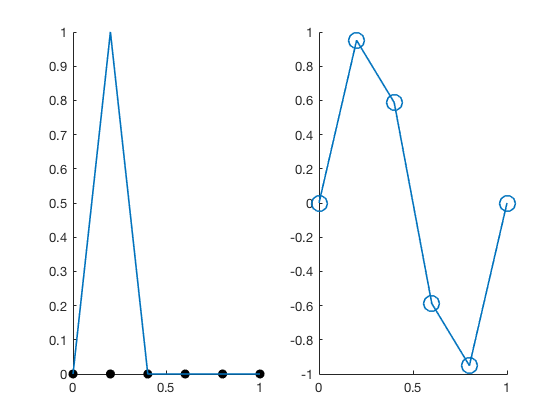
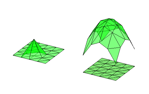
We take linear finite element spaces as an example. For each vertex $v_i$ of $\mathcal T$, let $\phi _i$ be the piecewise linear function such that $\phi _i(v_i)=1$ and $\phi _i(v_j)=0$ when $j\neq i$. The basis function in 1-D and 2-D is illustrated below. It is also called hat function named after the shape of its graph.
Then it is easy to see $\mathcal V_{\mathcal T}$ is spanned by the basis $\{ \phi_i \}_{i=1}^{N}$.
%% 1-D hat basis and a linear finite element functino
x = 0:1/5:1;
u = zeros(length(x),1);
u(2) = 1;
figure;
subplot(1,2,1); hold on;
plot(x,0,'k.','MarkerSize',18);
plot(x,u,'-','linewidth',1.2);
subplot(1,2,2); hold on;
u = sin(2*pi*x);
plot(x,u,'-o','linewidth',1.2,'MarkerSize',10);

% 2-D hat basis and a linear finite element functino
clf;
[node,elem] = squaremesh([-1,1,-1,1],0.5);
phi = zeros(size(node,1),1);
phi(12) = 1;
subplot(1,2,1);
showmesh(node,elem,'facecolor','none'); hold on;
showsolution(node,elem,phi,[30,26],'facecolor','g','facealpha',0.5,'edgecolor','k');
u = 3 - node(:,1).^2 - node(:,2).^2; % 3 - (x^2 + y^2)
% u = sin(node(:,1)).*cos(node(:,2));
subplot(1,2,2);
showmesh(node,elem); hold on;
showsolution(node,elem,u,[30,26],'facecolor','g','facealpha',0.5,'edgecolor','k');

Linear Algebraic System
For any function $v\in \mathcal V_{\mathcal T}$, there is a unique representation: $v=\sum_{i=1}^Nv_i\phi_i$. We thus can define an isomorphism $\mathcal V_{\mathcal T} \cong \mathbb R^N$ by
\[v=\sum _{i=1}^Nv_i\phi _i \longleftrightarrow \boldsymbol v=(v_1, \cdots, v_N)^{\intercal},\]and call $\boldsymbol v$ the coordinate vector of $v$ relative to the basis $\{ \phi_i \}_{i=1}^{N}$. Following the terminology in the elasticity theory, we introduce the stiffness matrix
\[\boldsymbol A=(a_{ij})_{N\times N}, \, \text{ with } \quad a_{ij}=a(\phi _j,\phi _i),\]for $a(\cdot,\cdot)$ from \eqref{eq:poisson-weak} and the load vector $\boldsymbol f=\{\langle f, \phi_k \rangle \}_{k=1}^{N}\in \mathbb{R}^{N}$. Then the coefficient vector $\boldsymbol u$ of $u$ can be obtained by solving the following linear algebraic system
\[\boldsymbol A\boldsymbol u = \boldsymbol f. \tag{3}\label{eq:system}\]It is straightforward to verify $\boldsymbol A$ is a symmetric and positive definite (SPD) matrix and thus the solution $\boldsymbol u$ exists and unique.
Numerical Examples
Numerical examples using the linear element for 2D Poisson equation is documented in
and more elements and equations can be found
Further Reading
-
Error estimate of the linear finite element method can be found in Introduction to Finite Element Methods
-
Assembling the matrix $\boldsymbol A$ and the vector $\boldsymbol f$ can be found in Progamming of Finite Element Methods
-
Fast solvers for solving the linear algebraic equation \eqref{eq:system} can be found in Multigrid Methods
Comments