Linear Element for Poisson Equation in 3D
This example is to show the rate of convergence of the linear finite element approximation of the Poisson equation on the unit cube:
\[- \Delta u = f \; \hbox{in } (0,1)^3\]for the following boundary conditions
- Non-empty Dirichlet boundary condition: $u=g_D \hbox{ on }\Gamma_D, \nabla u\cdot n=g_N \hbox{ on }\Gamma_N.$
- Pure Neumann boundary condition: $\nabla u\cdot n=g_N \hbox{ on } \partial \Omega$.
- Robin boundary condition: $g_R u + \nabla u\cdot n=g_N \hbox{ on }\partial \Omega$.
References:
- Quick Introduction to Finite Element Methods
- Introduction to Finite Element Methods
- Progamming of Finite Element Methods
Subroutines:
- Poisson3
- cubePoisson
- femPoisson3
- Poisson3femrate
The method is implemented in Poisson3 subroutine and tested in cubePoisson. Together with other elements (P1, P2,Q1,WG), femPoisson3 provides a concise interface to solve Poisson equation. The P1 element is tested in Poisson3femrate. This doc is based on Poisson3femrate.
P1 Linear Element
For the linear element on a simplex, the local basis functions are barycentric coordinate of vertices. The local to global pointer is elem. This is the simplest and default element for elliptic equations.
A local basis of P1
For $i = 1, 2, 3,4$, a local basis of the linear element space is given by the barycentric coordinate
\[\phi_i = \lambda_i, \quad \nabla \phi_i = \nabla \lambda_i = - \frac{1}{6|T|}\boldsymbol n_i\]| where $\boldsymbol n_i$ is the scaled (not unit) outwards normal direction with length $ | \boldsymbol n_i | = 2 | F_i | $, with $F_i$ being the face opposite to the i-th vertex. The gradient can be computed by |
[Dlambda,volume]= gradbasis3(node,elem);
See Finite Element Methods Section 2.1 for geometric explanation of the barycentric coordinate and Programming of Finite Element Methods in MATLAB for detailed explanation. For P1 element, the basic data structure node,elem is sufficient and displayed for the following coarse mesh.
node = [-1,-1,-1; 1,-1,-1; 1,1,-1; -1,1,-1; -1,-1,1; 1,-1,1; 1,1,1; -1,1,1];
elem = [1,2,3,7; 1,6,2,7; 1,5,6,7; 1,8,5,7; 1,4,8,7; 1,3,4,7];
clf; showmesh3(node,elem,[],'FaceAlpha',0.25);
view([-53,8]);
axis on
findelem3(node,elem);
findnode3(node);
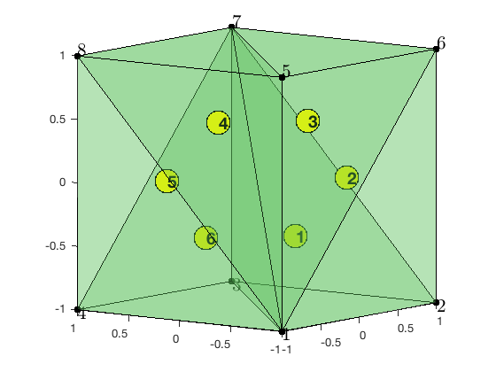
disp(elem);
     1     2     3     7
     1     6     2     7
     1     5     6     7
     1     8     5     7
     1     4     8     7
     1     3     4     7
Unlike 2-D case, to apply uniform refinement to obtain a fine mesh with good mesh quality, a different ordering of the inital mesh, which may violate the positive ordering, should be used. See 3 D Red Refinement.
Mixed boundary condition
%% Setting
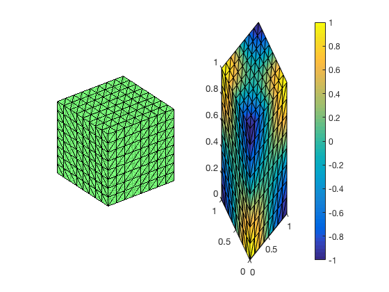
[node,elem] = cubemesh([0,1,0,1,0,1],0.5);
mesh = struct('node',node,'elem',elem);
option.L0 = 1;
option.maxIt = 4;
option.elemType = 'P1';
option.printlevel = 1;
option.plotflag = 1;
%% Non-empty Dirichlet boundary condition.
pde = sincosdata3;
mesh.bdFlag = setboundary3(node,elem,'Dirichlet','~(x==0)','Neumann','x==0');
femPoisson3(mesh,pde,option);
Multigrid V-cycle Preconditioner with Conjugate Gradient Method
#dof: 4913, #nnz: 23790, smoothing: (1,1), iter: 11, err = 3.72e-09, time = 0.14 s
Multigrid V-cycle Preconditioner with Conjugate Gradient Method
#dof: 35937, #nnz: 209374, smoothing: (1,1), iter: 11, err = 5.13e-09, time = 0.24 s
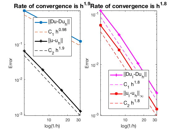
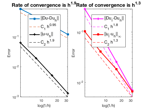
Table: Error
#Dof h ||u-u_h|| ||Du-Du_h|| ||DuI-Du_h|| ||uI-u_h||_{max}
125 2.500e-01 6.46061e-02 9.23927e-01 1.17911e-01 6.04325e-02
729 1.250e-01 1.86268e-02 4.80477e-01 3.91991e-02 1.95770e-02
4913 6.250e-02 4.86895e-03 2.42898e-01 1.06348e-02 5.17072e-03
35937 3.125e-02 1.23196e-03 1.21798e-01 2.72075e-03 1.31609e-03
Table: CPU time
#Dof Assemble Solve Error Mesh
125 1.09e-01 1.88e-02 6.00e-02 2.00e-02
729 4.94e-02 9.26e-04 3.00e-02 5.00e-02
4913 1.40e-01 1.41e-01 1.00e-01 1.00e-01
35937 1.45e+00 2.39e-01 8.50e-01 8.60e-01
Pure Neumann boundary condition
When pure Neumann boundary condition is posed, i.e., $-\Delta u =f$ in $\Omega$ and $\nabla u\cdot n=g_N$ on $\partial \Omega$, the data should be consisitent in the sense that $\int_{\Omega} f \, dx + \int_{\partial \Omega} g \, ds = 0$. The solution is unique up to a constant. A post-process is applied such that the constraint $\int_{\Omega}u_h dx = 0$ is imposed.
%% Pure Neumann boundary condition.
option.plotflag = 0;
mesh.bdFlag = setboundary3(node,elem,'Neumann');
femPoisson3(mesh,pde,option);
Multigrid V-cycle Preconditioner with Conjugate Gradient Method
#dof: 4913, #nnz: 32650, smoothing: (1,1), iter: 13, err = 2.43e-09, time = 0.076 s
Multigrid V-cycle Preconditioner with Conjugate Gradient Method
#dof: 35937, #nnz: 245018, smoothing: (1,1), iter: 14, err = 4.76e-09, time = 0.24 s
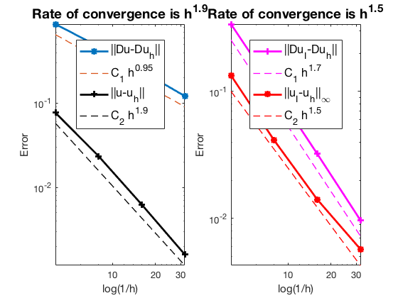
Table: Error
#Dof h ||u-u_h|| ||Du-Du_h|| ||DuI-Du_h|| ||uI-u_h||_{max}
125 2.500e-01 7.70680e-02 8.69504e-01 3.38890e-01 1.33687e-01
729 1.250e-01 2.35461e-02 4.70688e-01 1.05354e-01 4.13393e-02
4913 6.250e-02 6.27721e-03 2.41377e-01 3.23192e-02 1.41357e-02
35937 3.125e-02 1.59840e-03 1.21576e-01 9.72436e-03 5.74640e-03
Table: CPU time
#Dof Assemble Solve Error Mesh
125 3.73e-02 1.12e-03 1.00e-02 0.00e+00
729 1.32e-02 1.28e-02 1.00e-02 1.00e-02
4913 9.45e-02 7.62e-02 7.00e-02 1.00e-01
35937 1.47e+00 2.41e-01 8.40e-01 8.60e-01
Robin boundary condition
%% Pure Robin boundary condition.
pde = sincosRobindata3;
mesh.bdFlag = setboundary3(node,elem,'Robin');
femPoisson3(mesh,pde,option);
Multigrid V-cycle Preconditioner with Conjugate Gradient Method
#dof:     4913,  #nnz:    35729, smoothing: (1,1), iter: 11,   err = 2.75e-09,   time = 0.067 s
Multigrid V-cycle Preconditioner with Conjugate Gradient Method
#dof:    35937,  #nnz:   257313, smoothing: (1,1), iter: 11,   err = 8.49e-09,   time = 0.18 s
Table: Error
 #Dof       h        ||u-u_h||    ||Du-Du_h||   ||DuI-Du_h|| ||uI-u_h||_{max}

  125   2.500e-01   6.40633e-02   8.75746e-01   2.90399e-01   1.03297e-01
  729   1.250e-01   1.93507e-02   4.71714e-01   9.10331e-02   4.09455e-02
 4913   6.250e-02   5.14258e-03   2.41519e-01   2.57055e-02   1.83236e-02
35937   3.125e-02   1.30834e-03   1.21594e-01   6.98457e-03   6.58871e-03

Table: CPU time
 #Dof   Assemble     Solve      Error      Mesh

  125   5.16e-02   3.37e-04   0.00e+00   0.00e+00
  729   2.22e-02   3.12e-03   2.00e-02   1.00e-02
 4913   1.06e-01   6.72e-02   8.00e-02   7.00e-02
35937   1.18e+00   1.83e-01   8.60e-01   8.00e-01
Conclusion
The optimal rate of convergence of the H1-norm (1st order) and L2-norm (2nd order) is observed. The 2nd order convergent rate between two discrete functions $|\nabla (u_I - u_h)|$ is known as superconvergence.
MGCG converges uniformly in all cases.
Note that for Robin boundary condition, the order of the error in the maximum norm is not close to 2. Need to double check the code.
Comments