Linear Element for Poisson Equation in 2D
Intro
This example is to show the rate of convergence of the linear finite element approximation of the Poisson equation on the unit square:
\[- \Delta u = f \; \hbox{in } (0,1)^2\]for the following boundary conditions
- Non-empty Dirichlet boundary condition: $u=g_D \hbox{ on }\Gamma_D, \nabla u\cdot n=g_N \hbox{ on }\Gamma_N.$
- Pure Neumann boundary condition: $\nabla u\cdot n=g_N \hbox{ on } \partial \Omega$.
- Robin boundary condition: $g_R u + \nabla u\cdot n=g_N \hbox{ on }\partial \Omega$.
References
- Quick Introduction to Finite Element Methods
- Introduction to Finite Element Methods
- Progamming of Finite Element Methods
Subroutines
PoissonsquarePoissonfemPoissonPoissonfemrate
The method is implemented in Poisson subroutine and tested in squarePoisson. Together with other elements (P1, P2, P3, Q1), femPoisson provides a concise interface to solve Poisson equation. The P1 element is tested in Poissonfemrate. This doc is based on Poissonfemrate.
P1 Linear Element
For the linear element on a simplex, the local basis functions are
barycentric coordinate of vertices. The local to global pointer is
elem. This is the simplest and default element for elliptic equations.
A local basis of P1
For $i = 1, 2, 3$, a local basis of the linear element space is given by the barycentric coordinate
\[\phi_i = \lambda_i, \quad \nabla \phi_i = \nabla \lambda_i = - \frac{|e_i|}{2|T|}\boldsymbol n_i, \quad \int_T \nabla \phi_i\nabla \phi_j = \frac{1}{4|T|}\boldsymbol l_i \cdot \boldsymbol l_j\]where $e_i$ is the edge opposite to the $i$-th vertex and $\boldsymbol n_i$ is the unit outwards normal direction, and $\boldsymbol l_i$ is the edge vector of $e_i$.
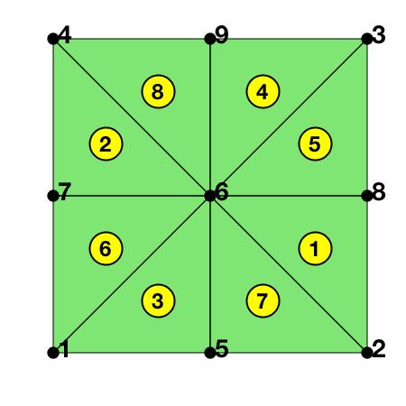
See Finite Element Methods Section 2.1 for geometric explanation of the barycentric coordinate and Programming of Finite Element Methods in MATLAB for detailed explanation. For P1 element, the basic data structure node,elem is sufficient and displayed for the following coarse mesh.
imatlab_export_fig('print-jpeg')
node = [0,0; 1,0; 1,1; 0,1];
elem = [2,3,1; 4,1,3];
[node,elem] = uniformbisect(node,elem);
figure('rend','painters','pos',[10 10 225 225])
showmesh(node,elem);
findnode(node);
findelem(node,elem);
display(elem);
elem =

     8     6     2
     7     6     4
     5     6     1
     9     6     3
     8     3     6
     7     1     6
     5     2     6
     9     4     6
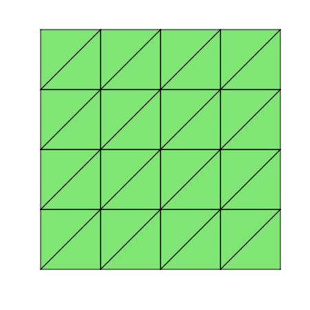
% Setting
[node,elem] = squaremesh([0,1,0,1],0.25);
mesh = struct('node',node,'elem',elem);
figure('rend','painters','pos',[10 10 225 225])
showmesh(node,elem);
option.L0 = 3;
option.maxIt = 4;
option.printlevel = 1;
Mixed boundary condition
option.plotflag = 0;
pde = sincosdata;
mesh.bdFlag = setboundary(node,elem,'Dirichlet','~(x==0)','Neumann','x==0');
femPoisson(mesh,pde,option);
Warning: File: /Dropbox/Math/Programming/ifem/solver/mg.m Line: 695 Column: 24
Defining "Di" in the nested function shares it with the parent function. In a future release, to share "Di" between parent and nested functions, explicitly define it in the parent function.
> In Poisson (line 233)
In femPoisson (line 65)
Multigrid V-cycle Preconditioner with Conjugate Gradient Method
#dof: 4225, #nnz: 19906, smoothing: (1,1), iter: 10, err = 1.55e-09, time = 0.11 s
Multigrid V-cycle Preconditioner with Conjugate Gradient Method
#dof: 16641, #nnz: 80770, smoothing: (1,1), iter: 10, err = 1.55e-09, time = 0.096 s
Multigrid V-cycle Preconditioner with Conjugate Gradient Method
#dof: 66049, #nnz: 325378, smoothing: (1,1), iter: 10, err = 1.47e-09, time = 0.2 s
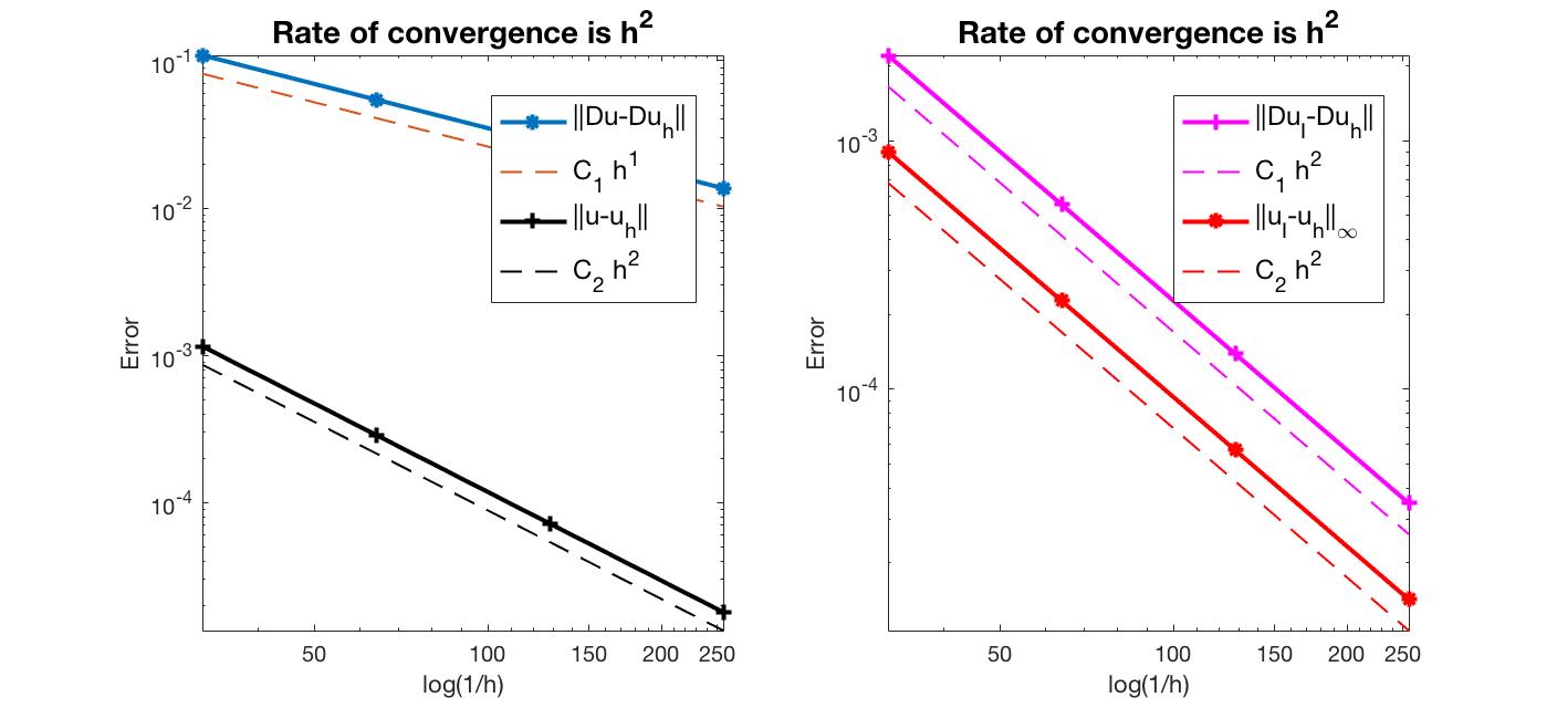
#Dof h ||u-u_h|| ||Du-Du_h|| ||DuI-Du_h|| ||uI-u_h||_{max}
1089 3.12e-02 1.15027e-03 1.08974e-01 2.21506e-03 9.04547e-04
4225 1.56e-02 2.88013e-04 5.45135e-02 5.54571e-04 2.26928e-04
16641 7.81e-03 7.20310e-05 2.72601e-02 1.38693e-04 5.67600e-05
66049 3.91e-03 1.80095e-05 1.36305e-02 3.46767e-05 1.41918e-05
#Dof Assemble Solve Error Mesh
1089 7.00e-02 1.36e-02 9.00e-02 1.00e-02
4225 3.00e-02 1.09e-01 4.00e-02 2.00e-02
16641 1.10e-01 9.62e-02 8.00e-02 6.00e-02
66049 4.00e-01 2.00e-01 2.30e-01 2.40e-01
Pure Neumann boundary condition
When pure Neumann boundary condition is posed, i.e., $-\Delta u =f$ in $\Omega$ and $\nabla u\cdot n=g_N$ on $\partial \Omega$, the data should be consisitent in the sense that $\int_{\Omega} f \, dx + \int_{\partial \Omega} g \, ds = 0$. The solution is unique up to a constant. A post-process is applied such that the constraint $\int_{\Omega}u_h dx = 0$ is imposed.
option.plotflag = 0;
pde = sincosNeumanndata;
pde = sincosdata;
mesh.bdFlag = setboundary(node,elem,'Neumann');
femPoisson(mesh,pde,option);
Multigrid V-cycle Preconditioner with Conjugate Gradient Method
#dof:     4225,  #nnz:    20860, smoothing: (1,1), iter: 12,   err = 1.43e-09,   time = 0.03 s
Multigrid V-cycle Preconditioner with Conjugate Gradient Method
#dof:    16641,  #nnz:    82684, smoothing: (1,1), iter: 12,   err = 6.33e-09,   time = 0.08 s
Multigrid V-cycle Preconditioner with Conjugate Gradient Method
#dof:    66049,  #nnz:   329212, smoothing: (1,1), iter: 13,   err = 2.40e-09,   time = 0.26 s

 #Dof       h       ||u-u_h||    ||Du-Du_h||   ||DuI-Du_h|| ||uI-u_h||_{max}

 1089   3.12e-02   1.29973e-03   1.08855e-01   5.80361e-03   3.86104e-03
 4225   1.56e-02   3.25931e-04   5.44960e-02   1.64867e-03   1.14414e-03
16641   7.81e-03   8.15520e-05   2.72576e-02   4.64515e-04   3.30465e-04
66049   3.91e-03   2.03927e-05   1.36301e-02   1.29765e-04   9.37017e-05

 #Dof   Assemble     Solve      Error      Mesh

 1089   5.00e-02   1.49e-03   2.00e-02   1.00e-02
 4225   2.00e-02   3.03e-02   3.00e-02   3.00e-02
16641   8.00e-02   7.97e-02   6.00e-02   5.00e-02
66049   4.00e-01   2.65e-01   3.00e-01   2.60e-01
Robin boundary condition
option.plotflag = 0;
pde = sincosRobindata;
mesh.bdFlag = setboundary(node,elem,'Robin');
femPoisson(mesh,pde,option);
Multigrid V-cycle Preconditioner with Conjugate Gradient Method
#dof: 4225, #nnz: 20865, smoothing: (1,1), iter: 10, err = 1.99e-09, time = 0.018 s
Multigrid V-cycle Preconditioner with Conjugate Gradient Method
#dof: 16641, #nnz: 82689, smoothing: (1,1), iter: 10, err = 2.33e-09, time = 0.062 s
Multigrid V-cycle Preconditioner with Conjugate Gradient Method
#dof: 66049, #nnz: 329217, smoothing: (1,1), iter: 10, err = 3.17e-09, time = 0.21 s
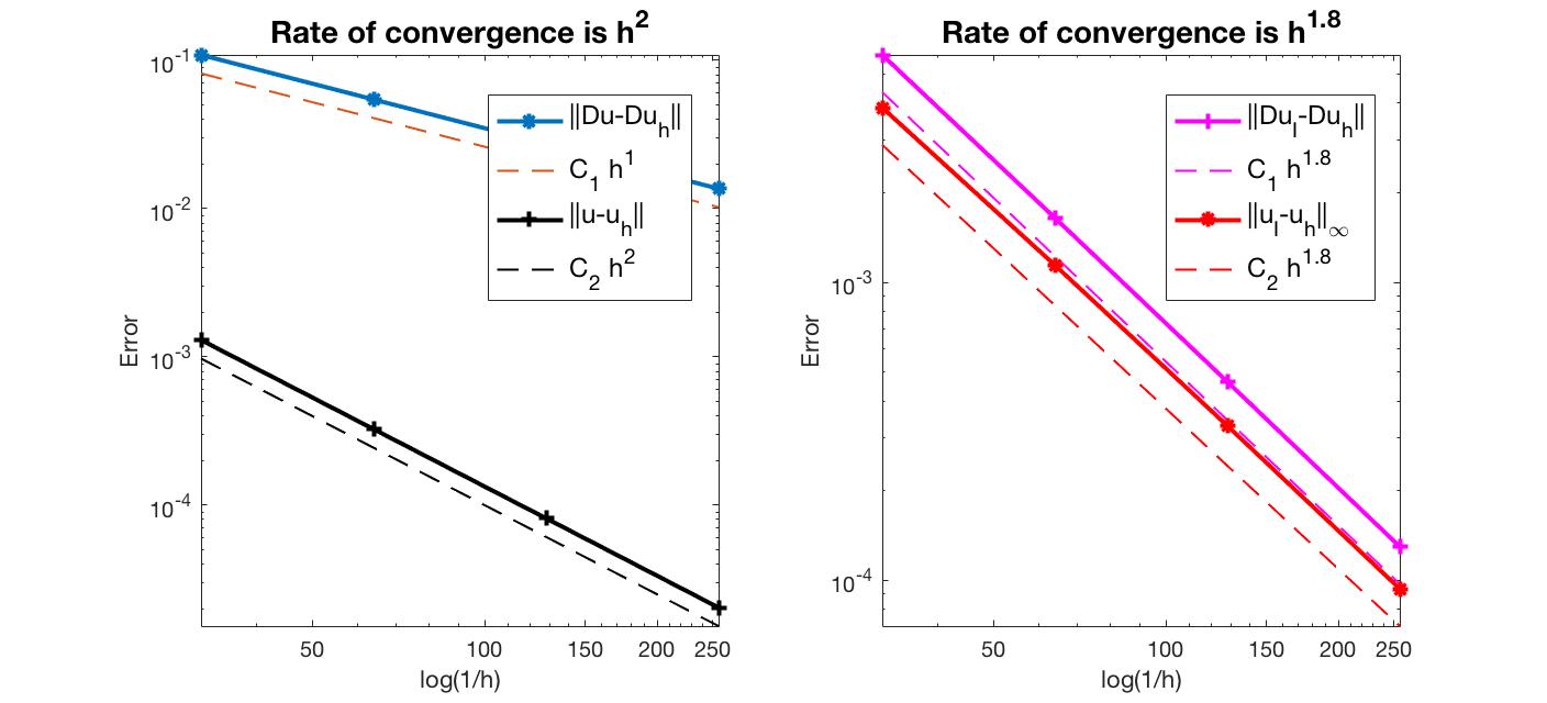
#Dof h ||u-u_h|| ||Du-Du_h|| ||DuI-Du_h|| ||uI-u_h||_{max}
1089 3.12e-02 4.92975e-03 4.34581e-01 2.56571e-02 8.30859e-03
4225 1.56e-02 1.24034e-03 2.17889e-01 6.44198e-03 2.08620e-03
16641 7.81e-03 3.10581e-04 1.09020e-01 1.61223e-03 5.22032e-04
66049 3.91e-03 7.76764e-05 5.45192e-02 4.03168e-04 1.30532e-04
#Dof Assemble Solve Error Mesh
1089 5.00e-02 1.39e-03 0.00e+00 1.00e-02
4225 2.00e-02 1.76e-02 2.00e-02 3.00e-02
16641 8.00e-02 6.17e-02 6.00e-02 5.00e-02
66049 4.90e-01 2.13e-01 2.50e-01 2.40e-01
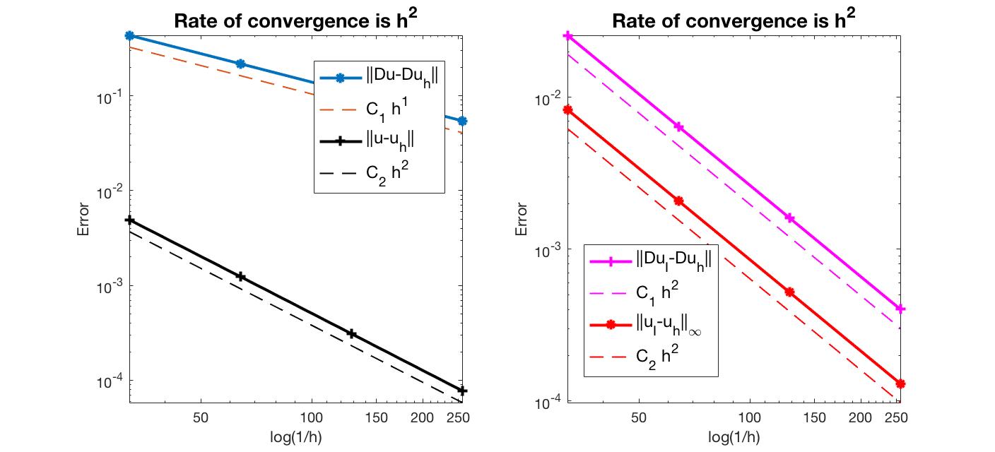
Conclusion
The optimal rate of convergence of the H1-norm (1st order) and L2-norm (2nd order) is observed. The 2nd order convergent rate between two discrete functions $|\nabla (u_I - u_h)|$ is known as superconvergence.
MGCG converges uniformly in all cases.
Comments