Linear Edge Element for Maxwell Equations in 3D
This example is to show the linear edge element approximation of the electric field of the time harmonic Maxwell equation.
\[\begin{aligned} \nabla \times (\mu^{-1}\nabla \times u) - \omega^2 \varepsilon \, u &= J \quad \text{ in } \quad \Omega, \\ n \times u &= n \times g_D \quad \text{ on } \quad \Gamma_D, \\ n \times (\mu^{-1}\nabla \times u) &= n \times g_N \quad \text{ on } \quad \Gamma_N. \end{aligned}\]based on the weak formulation
\[(\mu^{-1}\nabla \times u, \nabla \times v) - (\omega^2\varepsilon u,v) = (J,v) - \langle n \times g_N,v \rangle_{\Gamma_N}.\]Reference
- Finite Element Methods for Maxwell Equations
- Programming of Finite Element Methods for Maxwell Equations
Subroutines:
Maxwell1cubeMaxwell1femMaxwell3Maxwell1femrate
The method is implemented in Maxwell1 subroutine and tested in cubeMaxwell1. Together with other elements (ND0,ND1,ND2), femMaxwell3 provides a concise interface to solve Maxwell equation. The ND1 element is tested in Maxwell1femrate. This doc is based on Maxwell1femrate.
Data Structure
Use the function
[elem2dof,edge,elem2edgeSign] = dof3edge(elem);
to construct the pointer from element index to edge index. Read Dof on Edges in Three Dimensions for details.
node = [1,0,0; 0,1,0; 0,0,0; 0,0,1];
elem = [1 2 3 4];
localEdge = [1 2; 1 3; 1 4; 2 3; 2 4; 3 4];
imatlab_export_fig('print-png')  % Static png figures.
set(gcf,'Units','normal');
set(gcf,'Position',[0.25,0.25,0.25,0.25]);
showmesh3(node,elem);
view(-72,9);
findnode3(node);
findedge(node,localEdge,'all','vec');
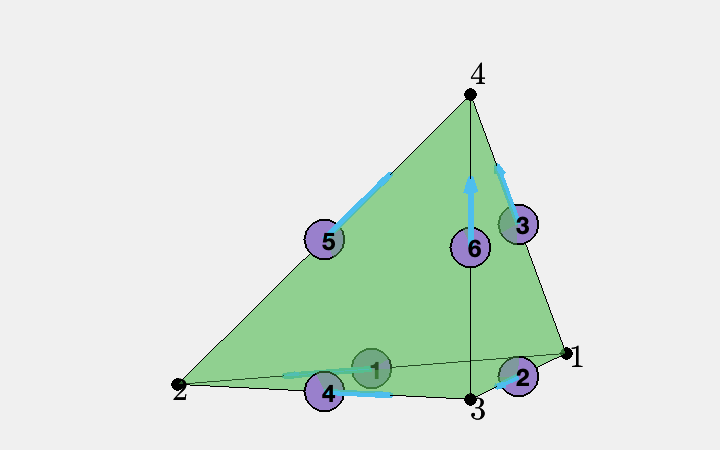
The six dofs associated to edges in a tetrahedron is sorted in the ordering [1 2; 1 3; 1 4; 2 3; 2 4; 3 4]. Here [1 2 3 4] are local indices of vertices.
Globally we use ascend ordering for each element and thus the orientation of the edge is consistent. No need of elem2edgeSign. Read Simplicial complex in three dimensions for more discussion of indexing, ordering and orientation.
Local Bases
Suppose [i,j] is the kth edge and i<j. The basis is given by
Inside one tetrahedron, the 6 bases functions along with their curl
corresponding to 6 local edges [1 2; 1 3; 1 4; 2 3; 2 4; 3 4] are
The additional 6 bases for the second family are:
\[\psi_k = \lambda_i\nabla \lambda_j + \lambda_j \nabla \lambda_i,\qquad \nabla \times \psi_k = 0.\] \[\psi_1 = \lambda_1\nabla\lambda_2 + \lambda_2\nabla\lambda_1,\] \[\psi_2 = \lambda_1\nabla\lambda_3 + \lambda_3\nabla\lambda_1,\] \[\psi_3 = \lambda_1\nabla\lambda_4 + \lambda_4\nabla\lambda_1,\] \[\psi_4 = \lambda_2\nabla\lambda_3 + \lambda_3\nabla\lambda_2,\] \[\psi_5 = \lambda_2\nabla\lambda_4 + \lambda_4\nabla\lambda_2,\] \[\psi_6 = \lambda_3\nabla\lambda_4 + \lambda_4\nabla\lambda_3.\]Degree of freedoms
Suppose [i,j] is the kth edge and i<j. The corresponding degree of freedom is
It is dual to the basis ${\phi_k}$ in the sense that
\[l_{\ell}(\phi _k) = \delta_{k,\ell}.\]The additional 6 degree of freedoms are:
\[l_k^1 (v) = 3\int_{e_k} v\cdot t(\lambda _i - \lambda_j) \, {\rm d}s \approx \frac{1}{2}[v(i) - v(j)]\cdot e_{k}.\]Dirichlet boundary condition
%% Setting
[node,elem] = cubemesh([-1,1,-1,1,-1,1],1);
mesh = struct('node',node,'elem',elem);
option.L0 = 1;
option.maxIt = 4;
option.elemType = 'ND1';
option.printlevel = 1;

%% Dirichlet boundary condition.
fprintf('Dirichlet boundary conditions. \n');
pde = Maxwelldata2;
bdFlag = setboundary3(node,elem,'Dirichlet');
femMaxwell3(mesh,pde,option);
Dirichlet boundary conditions.
#dof: 1208, Direct solver 0.1
#dof: 8368, Direct solver 0.23
Conjugate Gradient Method using HX preconditioner
#dof: 62048, #nnz: 1372268, iter: 37, err = 6.5415e-09, time = 1.6 s
Conjugate Gradient Method using HX preconditioner
#dof: 477376, #nnz: 11791756, iter: 36, err = 9.7991e-09, time = 11 s
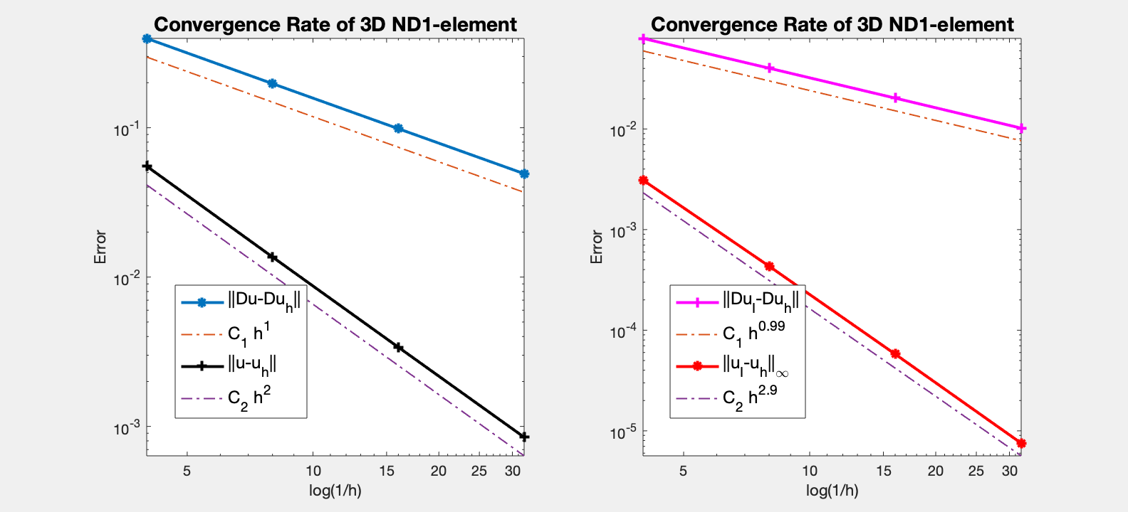
Table: Error
#Dof h ||u-u_h|| ||Du-Du_h|| ||DuI-Du_h|| ||uI-u_h||_{max}
1208 2.500e-01 5.52165e-02 3.96067e-01 7.95505e-02 3.10119e-03
8368 1.250e-01 1.36258e-02 1.97200e-01 4.02371e-02 4.33068e-04
62048 6.250e-02 3.39303e-03 9.84696e-02 2.02922e-02 5.78792e-05
477376 3.125e-02 8.47174e-04 4.92119e-02 1.01987e-02 7.53487e-06
Table: CPU time
#Dof Assemble Solve Error Mesh
1208 9.00e-02 1.00e-01 4.00e-02 1.00e-02
8368 1.20e-01 2.30e-01 7.00e-02 1.00e-02
62048 7.90e-01 1.56e+00 2.20e-01 5.00e-02
477376 6.15e+00 1.07e+01 1.71e+00 0.00e+00
Pure Neumann boundary condition
%% Pure Neumann boundary condition.
fprintf('Neumann boundary condition. \n');
option.plotflag = 0;
pde = Maxwelldata2;
mesh.bdFlag = setboundary3(node,elem,'Neumann');
femMaxwell3(mesh,pde,option);
Neumann boundary condition.
#dof:     1208, Direct solver 0.06
#dof:     8368, Direct solver 0.35
Conjugate Gradient Method using HX preconditioner
#dof:    62048,   #nnz:  1628576,   iter: 43,   err = 8.7403e-09,   time =    2 s
Conjugate Gradient Method using HX preconditioner
#dof:   477376,   #nnz: 12838720,   iter: 43,   err = 9.4520e-09,   time =   13 s
Table: Error
 #Dof        h        ||u-u_h||    ||Du-Du_h||   ||DuI-Du_h|| ||uI-u_h||_{max}

  1208   2.500e-01   2.41877e-02   3.90295e-01   9.93550e-02   1.88901e-02
  8368   1.250e-01   6.28974e-03   1.96199e-01   4.40961e-02   2.94393e-03
 62048   6.250e-02   1.59327e-03   9.82971e-02   2.10068e-02   4.34979e-04
477376   3.125e-02   4.00195e-04   4.91812e-02   1.03323e-02   6.24133e-05

Table: CPU time
 #Dof    Assemble     Solve      Error      Mesh

  1208   6.00e-02   6.00e-02   1.00e-02   0.00e+00
  8368   1.80e-01   3.50e-01   4.00e-02   1.00e-02
 62048   7.00e-01   1.95e+00   2.20e-01   4.00e-02
477376   5.47e+00   1.35e+01   1.69e+00   0.00e+00
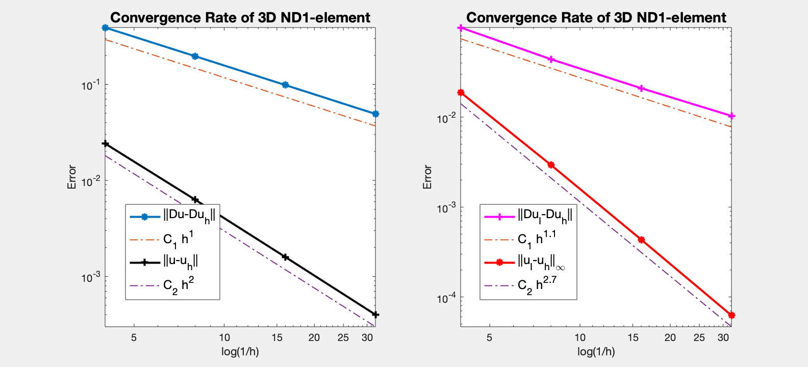
Conclusion
The H(curl)-norm is still 1st order but the L2-norm is improved to 2nd order.
MGCG using HX preconditioner converges uniformly in all cases.
Comments