Weak Galerkin Methods for Poisson Equation in 2D
This example is to show the rate of convergence of the lowest order Weak Galerkin finite element approximation of the Poisson equation on the unit square:
\[- \Delta u = f \; \hbox{in } (0,1)^2\]for the following boundary conditions
- Non-empty Dirichlet boundary condition: $u=g_D \hbox{ on }\Gamma_D, \nabla u\cdot n=g_N \hbox{ on }\Gamma_N.$
- Pure Neumann boundary condition: $\nabla u\cdot n=g_N \hbox{ on } \partial \Omega$.
- Robin boundary condition: $g_R u + \nabla u\cdot n=g_N \hbox{ on }\partial \Omega$.
References:
- Quick Introduction to Finite Element Methods
- Introduction to Finite Element Methods
- Progamming of Weak Galerkin Methods
Subroutines
PoissonWGsquarePoissonWGfemPoissonPoissonWGfemrate
The method is implemented in PoissonWG subroutine and can be tested in squarePoissonWG. Together with other elements (P1, P2, P3, Q1), femPoisson provides a concise interface to solve Poisson equation. The P2 element is tested in PoissonWGfemrate. This doc is based on PoissonWGfemrate.
The Lowest Order Weak Galerkin Element
The basis and the local matrices can be found in Progamming of Weak Galerkin Methods
Mixed boundary condition
%% Setting
[node,elem] = squaremesh([0,1,0,1],0.25);
mesh = struct('node',node,'elem',elem);
option.L0 = 2;
option.maxIt = 4;
option.printlevel = 1;
option.elemType = 'WG';
% Mixed boundary condition
pde = sincosdata;
mesh.bdFlag = setboundary(node,elem,'Dirichlet','~(x==0)','Neumann','x==0');
femPoisson(mesh,pde,option);
Multigrid V-cycle Preconditioner with Conjugate Gradient Method
#dof: 3136, #nnz: 14866, smoothing: (1,1), iter: 12, err = 2.67e-09, time = 0.1 s
Multigrid V-cycle Preconditioner with Conjugate Gradient Method
#dof: 12416, #nnz: 55426, smoothing: (1,1), iter: 12, err = 2.62e-09, time = 0.097 s
Multigrid V-cycle Preconditioner with Conjugate Gradient Method
#dof: 49408, #nnz: 238770, smoothing: (1,1), iter: 12, err = 2.57e-09, time = 0.18 s
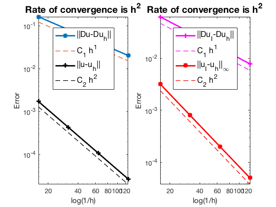
#Dof h ||u-u_h|| ||Du-Du_h|| ||DuI-Du_h|| ||uI-u_h||_{max}
800 6.250e-02 1.71814e-03 1.62480e-01 6.33304e-02 3.20790e-03
3136 3.125e-02 4.29635e-04 8.12679e-02 3.15253e-02 8.03198e-04
12416 1.562e-02 1.07415e-04 4.06374e-02 1.57451e-02 2.00838e-04
49408 7.812e-03 2.68539e-05 2.03191e-02 7.87036e-03 5.02182e-05
#Dof Assemble Solve Error Mesh
800 9.00e-02 1.41e-02 9.00e-02 1.00e-02
3136 7.00e-02 1.03e-01 4.00e-02 2.00e-02
12416 1.30e-01 9.69e-02 5.00e-02 1.00e-01
49408 3.00e-01 1.83e-01 1.10e-01 1.00e-01
Pure Neumann boundary condition
When pure Neumann boundary condition is posed, i.e., $-\Delta u =f$ in $\Omega$ and $\nabla u\cdot n=g_N$ on $\partial \Omega$, the data should be consisitent in the sense that $\int_{\Omega} f \, dx + \int_{\partial \Omega} g \, ds = 0$. The solution is unique up to a constant. A post-process is applied such that the constraint $\int_{\Omega}u_h dx = 0$ is imposed.
option.plotflag = 0;
pde = sincosNeumanndata;
mesh.bdFlag = setboundary(node,elem,'Neumann');
femPoisson(mesh,pde,option);
Multigrid V-cycle Preconditioner with Conjugate Gradient Method
#dof: 3136, #nnz: 15339, smoothing: (1,1), iter: 13, err = 4.49e-09, time = 0.066 s
Multigrid V-cycle Preconditioner with Conjugate Gradient Method
#dof: 12416, #nnz: 56235, smoothing: (1,1), iter: 14, err = 1.90e-09, time = 0.07 s
Multigrid V-cycle Preconditioner with Conjugate Gradient Method
#dof: 49408, #nnz: 240683, smoothing: (1,1), iter: 14, err = 3.96e-09, time = 0.24 s
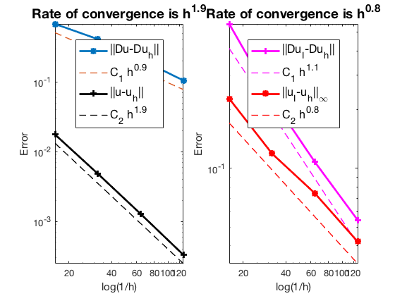
#Dof h ||u-u_h|| ||Du-Du_h|| ||DuI-Du_h|| ||uI-u_h||_{max}
800 6.250e-02 1.76689e-02 6.83050e-01 5.49515e-01 2.27492e-01
3136 3.125e-02 4.83700e-03 4.13444e-01 2.27292e-01 1.18952e-01
12416 1.562e-02 1.28283e-03 2.09935e-01 1.07773e-01 7.44907e-02
49408 7.812e-03 3.30853e-04 1.05872e-01 5.43084e-02 4.20973e-02
#Dof Assemble Solve Error Mesh
800 7.00e-02 1.42e-03 3.00e-02 0.00e+00
3136 1.00e-02 6.63e-02 2.00e-02 0.00e+00
12416 7.00e-02 7.00e-02 3.00e-02 1.00e-02
49408 2.70e-01 2.41e-01 1.30e-01 6.00e-02
Robin boundary condition
option.plotflag = 0;
pde = sincosRobindata;
mesh.bdFlag = setboundary(node,elem,'Robin');
femPoisson(mesh,pde,option);
Multigrid V-cycle Preconditioner with Conjugate Gradient Method
#dof: 3136, #nnz: 15344, smoothing: (1,1), iter: 12, err = 1.81e-09, time = 0.05 s
Multigrid V-cycle Preconditioner with Conjugate Gradient Method
#dof: 12416, #nnz: 56240, smoothing: (1,1), iter: 11, err = 9.88e-09, time = 0.051 s
Multigrid V-cycle Preconditioner with Conjugate Gradient Method
#dof: 49408, #nnz: 240688, smoothing: (1,1), iter: 12, err = 1.78e-09, time = 0.18 s
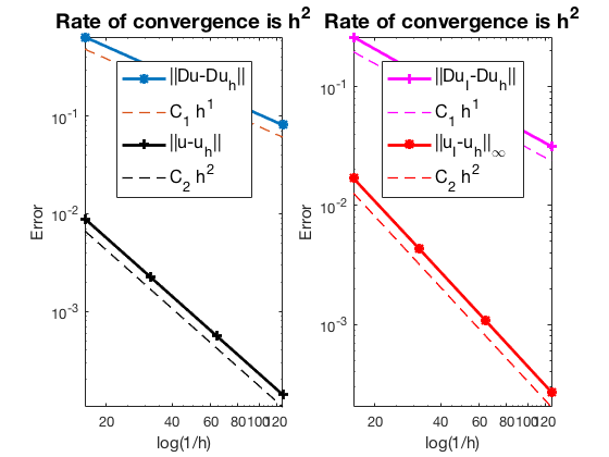
#Dof h ||u-u_h|| ||Du-Du_h|| ||DuI-Du_h|| ||uI-u_h||_{max}
800 6.250e-02 8.89017e-03 6.48648e-01 2.60943e-01 1.69325e-02
3136 3.125e-02 2.23100e-03 3.24914e-01 1.27079e-01 4.31205e-03
12416 1.562e-02 5.58282e-04 1.62530e-01 6.31035e-02 1.08242e-03
49408 7.812e-03 1.39604e-04 8.12741e-02 3.14968e-02 2.70809e-04
#Dof Assemble Solve Error Mesh
800 4.00e-02 1.37e-03 0.00e+00 1.00e-02
3136 2.00e-02 5.02e-02 1.00e-02 1.00e-02
12416 5.00e-02 5.15e-02 5.00e-02 1.00e-02
49408 2.10e-01 1.81e-01 1.00e-01 6.00e-02
Conclusion
The optimal rate of convergence of the H1-norm (1st order) and L2-norm (2nd order) is observed. No superconvergence for $|\nabla u_I - \nabla u_h|$.
MGCG converges uniformly in all cases.
Comments