BDM1-P0 Element for Poisson Equation in 2D
This example is to show the rate of convergence of the BDM1-P0 mixed finite element approximation of the Poisson equation on the unit square:
\[- \nabla (d \nabla) u = f \; \hbox{in } (0,1)^2\]for the following boundary conditions
- pure Dirichlet boundary condition: $u = g_D \text{ on } \partial \Omega$.
- Pure Neumann boundary condition: $d\nabla u\cdot n=g_N \text{ on } \partial \Omega$.
- mixed boundary condition: $u=g_D \text{ on }\Gamma_D, \nabla u\cdot n=g_N \text{ on }\Gamma_N.$
Find $(\sigma , u)$ in $H_{g_N,\Gamma_N}({\rm div},\Omega)\times L^2(\Omega)$ s.t.
\[(d^{-1}\sigma,\tau) + ({\rm div} \tau, u) = \langle \tau \cdot n, g_D \rangle_{\Gamma_D} \quad \forall \tau \in H_{0,\Gamma_N}(div,\Omega)\] \[(\mathrm{div}\, \sigma, v) = -(f,v) \quad \forall v \in L^2(\Omega)\]where
\[H_{g,\Gamma}(\mathrm{div},\Omega) = \{\sigma \in H(\mathrm{div}; \sigma \cdot n = g \text{ on } \Gamma \subset \partial\Omega \}.\]The unknown $\sigma = d\nabla u$ is approximated using the lowest order Brezzi-Douglas-Marini element (BDM1) and $u$ by piecewise constant element (P0).
References
Subroutines:
- PoissonBDM1
- squarePoissonBDM1
- mfemPoisson
- PoissonBDM1mfemrate
The method is implemented in PoissonBDM1 subroutine and tested in squarePoissonBDM1. Together with other elements (BDM1), mfemPoisson provides a concise interface to solve Poisson equation in mixed formulation. The RT0-P0 element is tested in PoissonBDM1mfemrate. This doc is based on PoissonBDM1mfemrate.
BDM1 Linear H(div) Element in 2D
We explain degree of freedoms and basis functions for Brezzi-Douglas-Marini element (BDM1) element on a triangle.
Asecond orientation
The dofs and basis depends on the orientation of the mesh. We shall use the asecond orientation, i.e., elem(t,1)< elem(t,2)< elem(t,3) not the positive orientation. Given an elem, the asecond orientation can be constructed by
[elem,bdFlag] = sortelem(elem,bdFlag); % ascend ordering
Note that bdFlag should be sorted as well.
The local edge is also asecond [2 3; 1 3; 1 2] so that the local orientation is consistent with the global one and thus no need to deal with the sign difference when the positive oritentation is used. Read Simplicial complex in two dimensions for more discussion of indexing, ordering and orientation.
node = [1,0; 1,1; 0,0];
elem = [1 2 3];
edge = [2 3; 1 3; 1 2];
figure;
subplot(1,2,1)
showmesh(node,elem);
findnode(node);
findedge(node,edge,'all','rotvec');
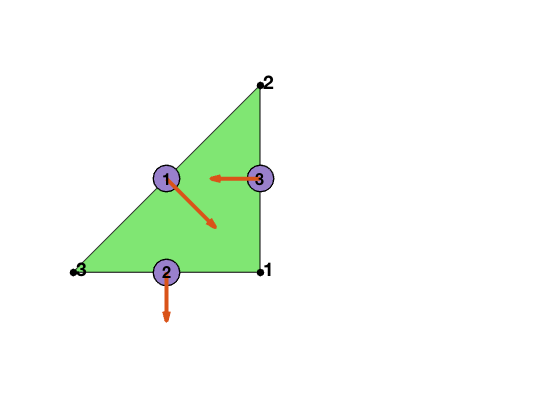
Local bases of BDM1 element
Suppose [i,j] is the k-th edge. The two dimensional curl is a rotated graident defined as $\nabla^{\bot} f = (-\partial_y f, \partial _x f).$ For RT0, the basis of this edge along with its divergence are given by
For BDM1, one more basis is added on this edge
\[\psi_k = \lambda_i \nabla^{\bot} \lambda_j + \lambda_j \nabla^{\bot} \lambda_i.\]Inside one triangular, the 6 bases corresponding to 3 local edges [2 3; 1 3; 1 2] are:
\[\phi_1 = \lambda_2 \nabla^{\bot} \lambda_3 - \lambda_3 \nabla^{\bot} \lambda_2, \quad \psi_1 = \lambda_2 \nabla^{\bot} \lambda_3 + \lambda_3 \nabla^{\bot} \lambda_2.\] \[\phi_2 = \lambda_1 \nabla^{\bot} \lambda_3 - \lambda_3 \nabla^{\bot} \lambda_1, \quad \psi_2 = \lambda_1 \nabla^{\bot} \lambda_3 + \lambda_3 \nabla^{\bot} \lambda_1.\] \[\phi_3 = \lambda_1 \nabla^{\bot} \lambda_2 - \lambda_2 \nabla^{\bot} \lambda_1, \quad \psi_3 = \lambda_1 \nabla^{\bot} \lambda_2 + \lambda_2 \nabla^{\bot} \lambda_1.\]Inside one triangle, we order the local bases in the following way:
\[\{\phi_1,~\,\phi_2,~\,\phi_3,~\,\psi_1,~\,\psi_2,~\, \psi_3.\}\]Note that $RT_0 \subset BDM_1$, and ${ \phi_1,~\,\phi_2,~\,\phi_3 }$ is the local bases for $RT_0$.
The first 3 dual bases are the line integral over orientated edges
\[d_i^{\phi}(u) = \int_{e_i} u \cdot n_i \, ds,\]and the second 3 dual bases are
\[d_{ij}^{\psi}(u) = 3 \int_{e_{i, j}} \boldsymbol{u} \cdot \boldsymbol{n}_{i, j}\left(\lambda_{i}-\lambda_{j}\right) \, ds,\]where $n_i = t_i^{\bot}$ is the rotation of the unit tangential vector of $e_i$ by $90^{\deg}$ counterclockwise.
It is straightforward to verify the “orthogonality”: \(d^{\phi}(\psi) = 0, \quad d^{\psi}(\phi) = 0, \quad d_i^{\phi}(\phi_j) = \delta_{ij}, \quad d_i^{\psi}(\psi_j) = \delta_{ij}.\)
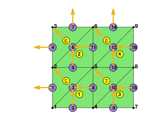
Local to global index map
Three local edges are locEdge = [2 3; 1 3; 1 2]. The pointer from the local to global index can be constructured by
[elem2edge,edge] = dofedge(elem);
[node,elem] = squaremesh([0 1 0 1], 0.5);
bdFlag = setboundary(node,elem,'Dirichlet');
[elem,bdFlag] = sortelem(elem,bdFlag);
showmesh(node,elem);
findnode(node);
findelem(node,elem);
[elem2edge,edge] = dofedge(elem);
findedge(node,edge,'all','rotvec');
display(elem2edge);
elem2edge =

  8�3 uint32 matrix

    8    3    2
   11    6    5
   15   10    9
   16   13   12
    5    3    1
    7    6    4
   12   10    8
   14   13   11
Assembling the matrix equation
We discuss several issues in the assembling.
Mass matrix
The mass matrix can be computed by
M = getmassmatvec(elem2edge,area,Dlambda,'BDM1');
divergence matrix
The ascend ordering orientation is not consistent with the induced orientation. The second edge would be [3 1] for the consistent orientation. So [1 -1 1] is used in the construction of div operator.
For triangle t, the basis for the constant function space is $p = 1$, the characteristic function. So in the computation of divergence operator, elemSign should be used to correct the sign. In the output of gradbasis, -Dlambda is always the outwards normal direction. The signed area could be negative but in the ouput, area is the absolute value (for the easy of integration on elements) and elemSign is used to record elements with negative area.
Note that $\nabla \cdot \psi = 0$ as $\psi = \nabla^{\bot} (\lambda_i\lambda_j)$ and $\nabla \cdot \nabla^{\bot} v = 0$. So it is simply a zero extension of that for RT0.
[Dlambda,area,elemSign] = gradbasis(node,elem);
B = icdmat(double(elem2edge),elemSign*[1 -1 1]);
NT = size(elem,1);
NE = double(max(elem2edge(:)));
B = [B sparse(NT,NE)];
disp(full(B));
  Columns 1 through 13

     0     1    -1     0     0     0     0     1     0     0     0     0     0
     0     0     0     0     1    -1     0     0     0     0     1     0     0
     0     0     0     0     0     0     0     0     1    -1     0     0     0
     0     0     0     0     0     0     0     0     0     0     0     1    -1
    -1     0     1     0    -1     0     0     0     0     0     0     0     0
     0     0     0    -1     0     1    -1     0     0     0     0     0     0
     0     0     0     0     0     0     0    -1     0     1     0    -1     0
     0     0     0     0     0     0     0     0     0     0    -1     0     1

  Columns 14 through 26

     0     0     0     0     0     0     0     0     0     0     0     0     0
     0     0     0     0     0     0     0     0     0     0     0     0     0
     0     1     0     0     0     0     0     0     0     0     0     0     0
     0     0     1     0     0     0     0     0     0     0     0     0     0
     0     0     0     0     0     0     0     0     0     0     0     0     0
     0     0     0     0     0     0     0     0     0     0     0     0     0
     0     0     0     0     0     0     0     0     0     0     0     0     0
    -1     0     0     0     0     0     0     0     0     0     0     0     0

  Columns 27 through 32

     0     0     0     0     0     0
     0     0     0     0     0     0
     0     0     0     0     0     0
     0     0     0     0     0     0
     0     0     0     0     0     0
     0     0     0     0     0     0
     0     0     0     0     0     0
     0     0     0     0     0     0
Boundary edges
Direction of boundary edges may not be the outwards normal direction of the domain since now elem is ascend orientation. edgeSign is introduced to record this inconsistency.
    edgeSign = ones(NE,1);
    idx = (bdFlag(:,1) ~= 0) & (elemSign == -1); % first edge is on boundary
    edgeSign(elem2edge(idx,1)) = -1;
    idx = (bdFlag(:,2) ~= 0) & (elemSign == 1);  % second edge is on boundary
    edgeSign(elem2edge(idx,2)) = -1;
    idx = (bdFlag(:,3) ~= 0) & (elemSign == -1); % third edge is on boundary
    edgeSign(elem2edge(idx,3)) = -1;
Test Examples
Mixed boundary condition
%% Setting
[node,elem] = squaremesh([0,1,0,1],0.25);
mesh = struct('node',node,'elem',elem);
option.L0 = 1;
option.maxIt = 4;
option.printlevel = 1;
option.elemType = 'BDM1';
pde = sincosNeumanndata;
%% Mix Dirichlet and Neumann boundary condition.
option.solver = 'uzawapcg';
mesh.bdFlag = setboundary(node,elem,'Dirichlet','~(x==0)','Neumann','x==0');
mfemPoisson(mesh,pde,option);
Uzawa-type MultiGrid Preconditioned PCG
#dof:      544,  #nnz:     3424, V-cycle:  1, iter: 15,   err = 5.39e-09,   time = 0.76 s
Uzawa-type MultiGrid Preconditioned PCG
#dof:     2112,  #nnz:    13760, V-cycle:  1, iter: 15,   err = 9.27e-09,   time = 0.22 s
Uzawa-type MultiGrid Preconditioned PCG
#dof:     8320,  #nnz:    55168, V-cycle:  1, iter: 16,   err = 3.40e-09,   time = 0.51 s
Uzawa-type MultiGrid Preconditioned PCG
#dof:    33024,  #nnz:   220928, V-cycle:  1, iter: 16,   err = 6.30e-09,   time =  1.9 s

 #Dof       h       ||u-u_h||    ||u_I-u_h||  ||sigma-sigma_h||||sigma-sigma_h||_{div}

  544   1.25e-01   1.33049e-01   4.89559e-02   3.51719e-01   1.01710e+01
 2112   6.25e-02   6.57965e-02   1.29683e-02   9.19906e-02   5.14701e+00
 8320   3.12e-02   3.27711e-02   3.29179e-03   2.32976e-02   2.58126e+00
33024   1.56e-02   1.63683e-02   8.26133e-04   5.84713e-03   1.29160e+00

 #Dof   Assemble     Solve      Error      Mesh

  544   3.00e-01   7.60e-01   2.40e-01   5.00e-02
 2112   1.40e-01   2.20e-01   1.30e-01   0.00e+00
 8320   9.00e-02   5.10e-01   6.00e-02   0.00e+00
33024   2.00e-01   1.91e+00   1.60e-01   3.00e-02
Pure Neumann boundary condition
In mixed formulation,the Neumann boundary condition for $d\nabla u$ becomes the Dirichlet boundary condiiton for $\sigma$. The space for $u$ is $L^2_0$ and thus one dof should be removed to have a non-singular system.
option.plotflag = 0;
option.solver = 'tri';
mesh.bdFlag = setboundary(node,elem,'Neumann');
mfemPoisson(mesh,pde,option);
Triangular Preconditioner Preconditioned GMRES
#dof:      544,  #nnz:     3047, V-cycle:  1, iter: 25,   err = 9.64e-09,   time = 0.17 s
Triangular Preconditioner Preconditioned GMRES
#dof:     2112,  #nnz:    12999, V-cycle:  1, iter: 26,   err = 6.74e-09,   time = 0.07 s
Triangular Preconditioner Preconditioned GMRES
#dof:     8320,  #nnz:    53639, V-cycle:  1, iter: 26,   err = 6.36e-09,   time =  0.2 s
Triangular Preconditioner Preconditioned GMRES
#dof:    33024,  #nnz:   217863, V-cycle:  1, iter: 25,   err = 7.62e-09,   time = 0.47 s

 #Dof       h       ||u-u_h||    ||u_I-u_h||  ||sigma-sigma_h||||sigma-sigma_h||_{div}

  544   1.25e-01   1.37562e-01   6.14647e-02   3.94535e-01   1.01710e+01
 2112   6.25e-02   6.59922e-02   1.46240e-02   1.02001e-01   5.14701e+00
 8320   3.12e-02   3.27830e-02   3.60849e-03   2.57227e-02   2.58126e+00
33024   1.56e-02   1.63694e-02   8.99021e-04   6.44489e-03   1.29160e+00

 #Dof   Assemble     Solve      Error      Mesh

  544   1.00e-02   1.70e-01   1.00e-02   0.00e+00
 2112   1.00e-02   7.00e-02   2.00e-02   0.00e+00
 8320   3.00e-02   2.00e-01   3.00e-02   1.00e-02
33024   1.60e-01   4.70e-01   1.20e-01   1.00e-02
Pure Dirichlet boundary condition
%% Pure Dirichlet boundary condition.
mesh.bdFlag = setboundary(node,elem,'Dirichlet');
mfemPoisson(mesh,pde,option);
Triangular Preconditioner Preconditioned GMRES
#dof:      544,  #nnz:     3552, V-cycle:  1, iter: 33,   err = 6.58e-09,   time = 0.09 s
Triangular Preconditioner Preconditioned GMRES
#dof:     2112,  #nnz:    14016, V-cycle:  1, iter: 32,   err = 6.14e-09,   time =  0.1 s
Triangular Preconditioner Preconditioned GMRES
#dof:     8320,  #nnz:    55680, V-cycle:  1, iter: 30,   err = 9.05e-09,   time = 0.32 s
Triangular Preconditioner Preconditioned GMRES
#dof:    33024,  #nnz:   221952, V-cycle:  1, iter: 29,   err = 7.69e-09,   time = 0.56 s

 #Dof       h       ||u-u_h||    ||u_I-u_h||  ||sigma-sigma_h||||sigma-sigma_h||_{div}

  544   1.25e-01   1.31849e-01   4.45750e-02   3.42158e-01   1.01710e+01
 2112   6.25e-02   6.56419e-02   1.19208e-02   8.96275e-02   5.14701e+00
 8320   3.12e-02   3.27516e-02   3.03288e-03   2.27060e-02   2.58126e+00
33024   1.56e-02   1.63659e-02   7.61593e-04   5.69922e-03   1.29160e+00

 #Dof   Assemble     Solve      Error      Mesh

  544   1.00e-02   9.00e-02   1.00e-02   1.00e-02
 2112   2.00e-02   1.00e-01   2.00e-02   0.00e+00
 8320   6.00e-02   3.20e-01   6.00e-02   0.00e+00
33024   1.60e-01   5.60e-01   1.50e-01   1.00e-02
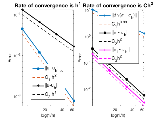
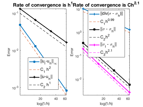
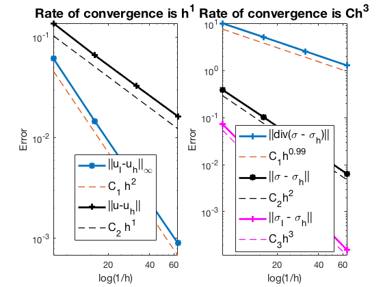
Conclusion
The optimal rates of convergence for $u$ and $\sigma$ are observed, namely, 1st order for L2 norm of u and H(div) norm of $\sigma$. The 2nd order convergent rates between two discrete functions $|u_I - u_h|$ is known as superconvergence. Compare with RT0, the L2 norm of $\sigma$ is 2nd order.
Triangular preconditioned GMRES (the default solver) and Uzawa preconditioned CG converges uniformly in all cases. Traingular preconditioner is two times faster than PCG although GMRES is used and iteration steps are doubled.
Comments