Project: Multigrid Methods
In this project we will learn three ways of implementating multigrid methods: from matrix-free to matrix-only depending on how much information on the grid and PDE is provided.
Reference
Multigrid on Uniform Grids for Poisson Equations
We consider the linear finite element or equivalently 5-point stencil discretization of the Poisson equation on a uniform grid of $[0,1]^2$ with size $h$. For simplicity, we assume $h = 1/2^L$ and zero Dirichlet bounary condition.
Step 1. Smoother
-
Code the weighted Jacobi and the Gauss-Seidel smoother using the matrix-free style; see Project: Finite Difference Methods
-
Check convergence of the Gauss-Seidel smoother by solving $-\Delta u = 1$ in $(0,1)^2$ with zero Dirichlet boundary condition. Plot the error in a suitable norm vs the iteration step for a fixed
h = 1/16. -
Change
hfrom1/4to1/128and compare the iteration steps to drive the relative error below the discretiztion error $h^2$. -
Choose a random initial guess and plot the error function on the grid
h = 1/16for the first 3 steps. -
(Optional) Code the red-black Gauss-Seidel.
Step 2. Two-Grid method
-
Figure out the index map between fine grid with size
hand coarse grid with size2h. For example,(i,j)in the coarse grid is(2*i-1,2*j-1)in the fine grid. -
Code the bilinear prolongation and restriction using the index map. Be carefuly on the value on the boundary points.
-
Code the two-grid method. On the fine grid, apply m times G-S iteration and then restrict the updated residual to the coarse grid. On the coarse grid, use G-S iteration or the direct method to solve the equation below the discretization error. Then prolongates the correction to the fine grid and apply additional m G-S iterations.
-
Use the two-grid method as an iteration to solve the Poisson equation.
-
Change
hfrom1/4to1/128and compare the iterations of two-grid methods for different h.
Step 3. V-cycle Multi-grid method
Choose one of the following approach to implement the MG.
-
(Recrusive way) Apply the two-grid method to the coarse grid problem in Step 2.
-
(Non-recrusive way) Follow the description of SSC in lecture notes to implement V-cycle.
- Use the Vcycle as an iteration to solve the Poisson equation, i.e.,
while relative residual < tol u = u + Vcycle(r,J); % correction form or u = Vcycle(u,J); % direct update form end - Change
hfrom1/4to1/128and check the iterations and cpu time of MG.
Multigrid on Hierarchical Grids
We consider the linear finite element discretization of the Poisson equation on grids obtained by uniform refinement of a coarse grid.
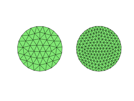
[node,elem] = circlemesh(0,0,1,0.25);
subplot(1,2,1); showmesh(node,elem);
[node,elem] = uniformrefine(node,elem);
subplot(1,2,2); showmesh(node,elem);
- Min quality 0.8507 - Mean quality 0.9612 - Uniformity 3.93%

Step 1. Hierarchical Meshes
Generate the initial grid by
[node,elem] = circlemesh(0,0,1,0.25);
-
Refine the initial mesh
Jtimes to get the finest mesh. To get a mesh of the disk, the boundary nodes should be projected onto the unit circle. -
Construct
HBin two ways. Either from the output ofuniformrefineduring the refinement or calluniformcoarsenredfrom the finest mesh.
Step 2. Transfer Operator and Smoothers
-
Assemble the stiffness matrix A in the finest mesh.
-
Construct prolongation and restriction matrices using
HB. -
Compute stiffness matrix in each level by the triple product.
-
Store the smoother tril(A) and triu(A) in each level.
Step 3. V-cycle Multigrid
-
Follow the lecture notes Introduction to Multigrid method to implement the non-recrusive V-cycle.
Be careful on the boundary nodes. Restrict smoothing to interiori nodes only and enforce the residual on boundary nodes to be zero.
-
For one single grid, say
J = 4, show the decrease of the residual in certain norm for each iteration of the multigrid method. -
Test V-cycle MG for
J = 3:6. List iteration steps and cpu time.
Algebraic Multigrid Methods
We consider solving an SPD matrix equation Ax = b, where A could be
obtained as the finite element discretization on a unstructured grids. A
coarsening of the graph of A is needed and restriction and prolongation
can be constructued based on the coarsening.
Step 1 Matrix
-
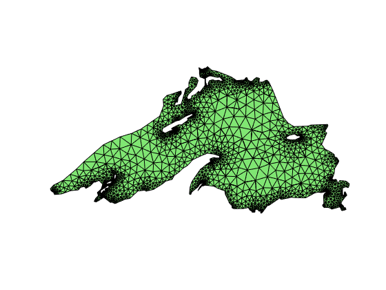
Load the
lakemesh.matin ifem/data. -
Assemble the stiffness matrix on this mesh and take the submatrix associated to interior nodes only.
The mesh is only used to generate the matrix. In the later step, only the generated matrix is used.
load lakemesh.mat;
figure; clf; showmesh(node,elem);
A = assemblematrix(node,elem);

Step 2 Coarsening
Use coarsenAMGc to get a set of coarse nodes.
help coarsenAMGc
  COARSENAMGC coarsen the graph of A.

  isC = coarsenAMGc(A) terturns a logical array to make a set of nodes as
  the coarse ndoes based on As, a strong connectness matrix modified from
  A. The strong connectness is slightly different with the standard
  definition.

  [isC,As] = coarsenAMGc(A,theta) accepts the parameter theta to define the
  strong connectness. The default setting is theta = 0.025. It also outputs
  the strong connectness matrix As which could be used in the constrction
  of prolongation and restriction.

  Example
    load lakemesh
    A = assemblematrix(node,elem);
    [isC,As] = coarsenAMGc(A);

  See also: coarsenAMGrs, interpolationAMGs, amg

  Reference page in Help browser
        <a href="matlab:ifem coarseAMGdoc">coarsenAMGdoc</a>

  Copyright (C) Long Chen. See COPYRIGHT.txt for details.
Step 3 Transfer Operator and Smoothers
Use interpolationAMGs to get restriction and prolongation operators.
help interpolationAMGs
  INTERPOLATIONAMGS construct prolongation and restriction matrices

  [Pro,Res] = interpolatoinAMGs(A,isC) construct prolongation and
  restriction matrices use standard matrix-dependent interpolation.

  In the input, A is a SPD matrix and isC is a logical array to indicate
  nodes in coarse matrix. In the output Pro and Res are prolongation and
  restriction matrices satisfying Res = Pro'.

  The submatrix A_{cf} is used to construct the interpolation of values on
  fine nodes from that of coarse nodes. The weight is normalized to
  preserve the constant.

  Example
    load lakemesh
    A = assemblematrix(node,elem);
    [isC,As] = coarsenAMGc(A);
    [Pro,Res] = interpolationAMGs(As,isC);

  See also: coarsenAMGc, amg

  Copyright (C) Long Chen. See COPYRIGHT.txt for details.
Step 4. V-cycle Multigrid used with PCG
Follow the Step 3 in part 2 to code a V-cycle. Then use the V-cycle as a preconditioner in PCG.
Test the robustness of the solver, apply uniformrefine to a mesh and
generate corresponding matrix. List the iteration steps and CPU time for
different size of matrices.
Comments