Data Structure: Boundary Conditions
We use bdFlag(1:NT,1:3) to record the type of three edges of each
triangle. Similarly in 3-D, we use bdFlag(1:NT,1:4) to record the type
of four faces of each tetrahedron. The value is the type of boundary
condition:
- 0: non-boundary, i.e., an interior edge or face.
- 1: first type, i.e., a Dirichlet boundary edge or face.
- 2: second type, i.e., a Neumann boundary edge or face.
- 3: third type, i.e., a Robin boundary edge or face.
For a boundary edge/face, the type is 0 means homogenous Neumann boundary condition (zero flux).
The function setboundary is to set up the bdFlag matrix for a 2-D
triangulation and setboundary3 for a 3-D triangulation. Examples
bdFlag = setboundary(node,elem,'Dirichlet','abs(x) + abs(y) == 1','Neumann','y==0');
bdFlag = setboundary3(node,elem,'Dirichlet','(z==1) | (z==-1)');
Local Labeling of Edges and Faces
We label three edges of a triangle such that bdFlag(t,i) is the edge
opposite to the i-th vertex. Similarly bdFlag(t,i) is the face opposite
to the i-th vertex for a tetrahedron.
node = [1,0; 1,1; 0,0];
elem = [1 2 3];
locEdge = [2 3; 3 1; 1 2];
showmesh(node,elem);
findnode(node);
findedge(node,locEdge,'all','vec');
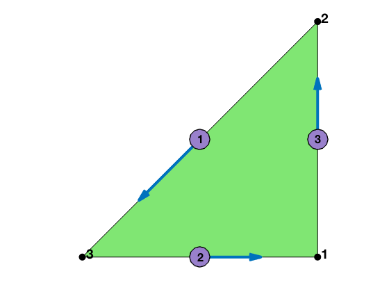
The ordering of edges is specified by locEdge. If we use locEdge = [2 3; 1 3; 1 2], we get asecond orientation of edges.
Changing Ordering
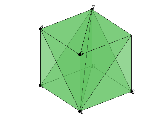
If we change the ordering of elem, the corresponding local faces are changed. Therefore when we sort the elem, we should sort the bdFlag simutaneously. For example, sort(elem,2) sorts the elem only, and leave bdFlag unchanged. Use sortelem (2D) or sortelem3 (3D) to sort elem and bdFlag at the same time.
[node,elem] = cubemesh([-1,1,-1,1,-1,1],2);
bdFlag = setboundary3(node,elem,'Dirichlet','x==1','Neumann','x~=1');
figure(2); clf;
showmesh3(node,elem);
display(elem); display(bdFlag);
findnode3(node,[1,2,3,4,5,7,8]);
display('change to ascend ordering');
[elem,bdFlag] = sortelem3(elem,bdFlag)
elem =

     1     2     3     7
     1     4     3     7
     1     5     6     7
     1     5     8     7
     1     2     6     7
     1     4     8     7


bdFlag =
   6x4 uint8 matrix

   1   0   0   2
   2   0   0   2
   2   0   0   2
   2   0   0   2
   1   0   0   2
   2   0   0   2

change to ascend ordering

elem =

     1     2     3     7
     1     3     4     7
     1     5     6     7
     1     5     7     8
     1     2     6     7
     1     4     7     8


bdFlag =
   6x4 uint8 matrix

   1   0   0   2
   2   0   0   2
   2   0   0   2
   2   0   2   0
   1   0   0   2
   2   0   2   0
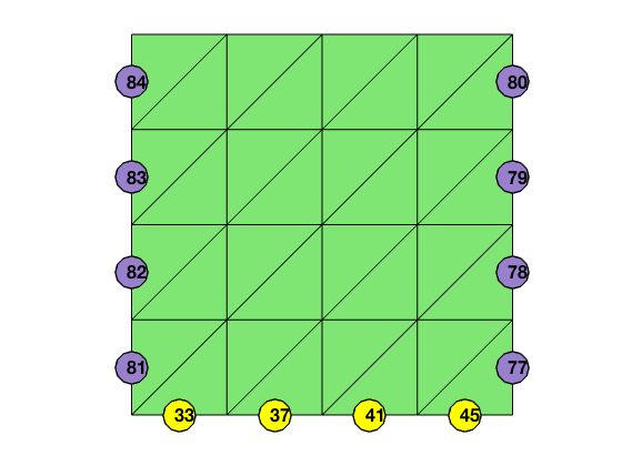
Extract Boundary Edges and Faces
We may extract boundary edges for a 2-D triangulation from bdFlag from the following code. If elem is sorted counterclockwise, the boundary edges inherits the orientation. See also findboundary and findboundary3.
[node,elem] = squaremesh([0 1 0 1], 0.25);
showmesh(node,elem); hold on;
bdFlag = setboundary(node,elem,'Dirichlet','x == 0 | x ==1','Neumann','y==0');
totalEdge = [elem(:,[2,3]); elem(:,[3,1]); elem(:,[1,2])];
Dirichlet = totalEdge(bdFlag(:) == 1,:);
findedge(node,totalEdge,bdFlag(:) == 1);
Neumann = totalEdge(bdFlag(:) == 2,:);
findedge(node,totalEdge,bdFlag(:) == 2,'MarkerFaceColor','y');
Or simply call
[bdNode,bdEdge,isBdNode] = findboundary(elem,bdFlag);
To find the outward normal direction of the boundary face, we use gradbasis3 to get Dlambda(t,:,k) which is the gradient of $\lambda_k$. The outward normal direction of the kth face can be obtained by -Dlambda(t,:,k) which is independent of the ordering and orientation of elem.
Dlambda = gradbasis3(node,elem);
T = auxstructure3(elem);
elem2face = T.elem2face;
face = T.face;
NF = size(face,1);
if ~isempty(bdFlag)
    % Find Dirchelt boundary faces and nodes
    isBdFace = false(NF,1);
    isBdFace(elem2face(bdFlag(:,1) == 1,1)) = true;
    isBdFace(elem2face(bdFlag(:,2) == 1,2)) = true;
    isBdFace(elem2face(bdFlag(:,3) == 1,3)) = true;
    isBdFace(elem2face(bdFlag(:,4) == 1,4)) = true;
    DirichletFace = face(isBdFace,:);
    % Find outwards normal direction of Neumann boundary faces
    bdFaceOutDirec = zeros(NF,3);
    bdFaceOutDirec(elem2face(bdFlag(:,1) == 2,1),:) = -Dlambda(bdFlag(:,1) == 2,:,1);
    bdFaceOutDirec(elem2face(bdFlag(:,2) == 2,2),:) = -Dlambda(bdFlag(:,2) == 2,:,2);
    bdFaceOutDirec(elem2face(bdFlag(:,3) == 2,3),:) = -Dlambda(bdFlag(:,3) == 2,:,3);
    bdFaceOutDirec(elem2face(bdFlag(:,4) == 2,4),:) = -Dlambda(bdFlag(:,4) == 2,:,4);
end
% normalize the boundary face outwards direction
vl = sqrt(dot(bdFaceOutDirec,bdFaceOutDirec,2));
idx = (vl==0);
NeumannFace = face(~idx,:);
bdFaceOutDirec(idx,:) = [];
vl(idx) = [];
bdFaceOutDirec = bdFaceOutDirec./[vl vl vl];
display(DirichletFace);
display(NeumannFace);
display(bdFaceOutDirec);
DirichletFace =

  2x3 uint32 matrix

   2   3   7
   2   6   7

NeumannFace =
  10x3 uint32 matrix

   1   2   3
   1   2   6
   1   3   4
   1   4   8
   1   5   6
   1   5   8
   3   4   7
   4   7   8
   5   6   7
   5   7   8


 bdFaceOutDirec =

     0     0    -1
     0    -1     0
     0     0    -1
    -1     0     0
     0    -1     0
    -1     0     0
     0     1     0
     0     1     0
     0     0     1
     0     0     1
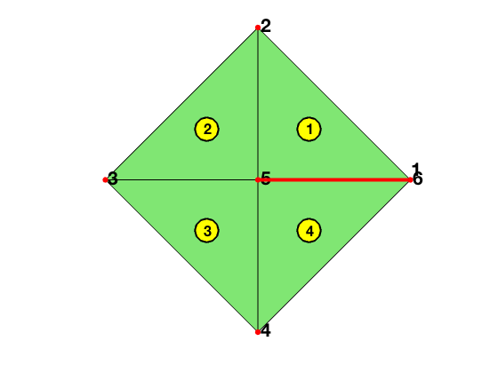
Example: Crack Domain
node = [1,0; 0,1; -1,0; 0,-1; 0,0; 1,0];        % nodes
elem = [5,1,2; 5,2,3; 5,3,4; 5,4,6];            % elements
elem = label(node,elem);                        % label the mesh
figure;
showmesh(node,elem);                            % plot mesh
findelem(node,elem);                            % plot element indices
findnode(node,2:6);                             % plot node indices
text(node(6,1),node(6,2)+0.075,int2str(1),'FontSize',16,'FontWeight','bold');
hold on;
plot([node(1,1),node(5,1)], [node(1,2),node(5,2)],'r-', 'LineWidth',3);
bdFlag = setboundary(node,elem,'Dirichlet'); % Dirichlet boundary condition
display(elem)
display(bdFlag)
elem =

     5     1     2
     5     2     3
     5     3     4
     5     4     6
bdFlag =
1 0 1
1 0 0
1 0 0
1 1 0
bdFlag = setboundary(node,elem,'Dirichlet','abs(x) + abs(y) == 1','Neumann','y==0');
display(bdFlag)
bdFlag =

    1    0    2
    1    0    0
    1    0    0
    1    2    0
The red line represents a crack. Although node 1 and node 6 have the same coordinate (1,0), they are different nodes and used in different triangles. An array u with u(1)~=u(6) represents a discontinous function. Think about a paper cut through the red line.
Example: Prism Domain
node = [-1,-1,-1; 1,-1,-1; 1,1,-1; -1,1,-1; -1,-1,1; 1,-1,1; 1,1,1; -1,1,1];
elem = [1,2,3,7; 1,6,2,7; 1,5,6,7];
elem = label3(node,elem);
figure;
showmesh3(node,elem);
view([-53,8]);
findnode3(node,[1 2 3 5 6 7]);
findelem3(node,elem);
bdFlag = setboundary3(node,elem,'Dirichlet','(z==1) | (z==-1)');
display(elem)
display(bdFlag)
elem =

     1     7     2     3
     1     7     6     2
     1     7     5     6
bdFlag =
0 1 0 0
0 0 0 0
1 0 0 0
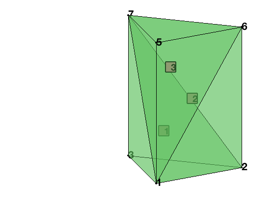
The top and bottom of the prism is set as Dirichlet boundary condition and other faces are zero flux boundary condition. Note that if the i-th face of t is on the boundary but bdFlag(t,i)=0, it is equivalent to use homogenous Neumann boundary condition (zero
flux).
Remark
It would save storage if we record boundary edges or faces only. The current data structure is convenient for the local refinement and coarsening since the boundary can be easily updated along with the change of elements. The matrix bdFlag is sparse but a dense matrix is used. We do not save bdFlag as a sparse matrix since updating sparse matrices is time-consuming. Instead we set up the type of bdFlag to uint8 to minimize the waste of memory.
Comments