Quadratic Element for Poisson Equation in 3D
This example is to show the rate of convergence of the linear finite element approximation of the Poisson equation on the unit square:
\[- \Delta u = f \; \hbox{in } (0,1)^3\]for the following boundary conditions
- Non-empty Dirichlet boundary condition: $u=g_D \hbox{ on }\Gamma_D, \nabla u\cdot n=g_N \hbox{ on }\Gamma_N.$
- Pure Neumann boundary condition: $\nabla u\cdot n=g_N \hbox{ on } \partial \Omega$.
- Robin boundary condition: $g_R u + \nabla u\cdot n=g_N \hbox{ on }\partial \Omega$.
References:
- Quick Introduction to Finite Element Methods
- Introduction to Finite Element Methods
- Progamming of Finite Element Methods
Subroutines:
- Poisson3P2
- cubePoissonP2
- femPoisson3
- Poisson3P2femrate
The method is implemented in Poisson3P2 subroutine and tested in cubePoissonP2. Together with other elements (P1, P2,Q1,WG), femPoisson3 provides a concise interface to solve Poisson equation. The P2 element is tested in Poisson3P2femrate. This doc is based on Poisson3P2femrate.
P2 Quadratic Element
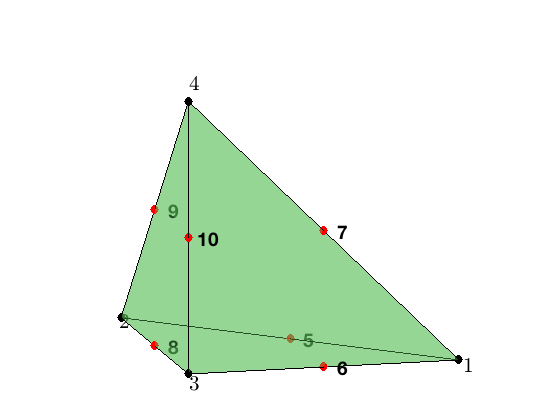
For the quadratic element on a tetrahedron, the local basis functions can be written in terms of barycentric coordinates. The 10 dofs is displayed below. The first 4 are associated to the vertices and 6 to the middle points of 6 edges.
Given a mesh, the required data structure can be constructured by
[elem2dof,edge,bdDof] = dof3P2(elem)
Local indexing
The tetrahedron consists of four vertices indexed as [1 2 3 4]. Each tetrahedron contains four faces and six edges. They can be indexed as
locFace = [2 3 4; 1 4 3; 1 2 4; 1 3 2];
locEdge = [1 2; 1 3; 1 4; 2 3; 2 4; 3 4];
In locFace, the i-th face is opposite to the i-th vertices and the orientation is induced from the tetrahedronthus this is called opposite indexing. In locEdge, it is the lexicographic indexing which is induced from the lexicographic ordering of the six edges.
node = [1,0,0; 0,1,0; 0,0,0; 0,0,1];
elem = [1 2 3 4];
locEdge = [1 2; 1 3; 1 4; 2 3; 2 4; 3 4];
showmesh3(node,elem);
view(-14,12);
findnode3(node);
findedgedof3(node,locEdge);
Boundary dof
When implement boundary conditions, we need to find the d.o.f associated to boundary faces. For example, for Neumann boundary conditions, it can be found by
           bdFace2dof = [elem2dof(bdFlag(:,1) == 2,[2,3,4,10,9,8]); ...
                         elem2dof(bdFlag(:,2) == 2,[1,4,3,10,6,7]); ...
                         elem2dof(bdFlag(:,3) == 2,[1,2,4,9,7,5]); ...
                         elem2dof(bdFlag(:,4) == 2,[1,3,2,8,5,6])];
A local basis
The 10 Lagrange-type bases functions are denoted by $\phi_i, i=1:10$. In barycentric coordinates, they are
\[\phi_1 = \lambda_1(2\lambda_1 -1),\quad \nabla \phi_1 = \nabla \lambda_1(4\lambda_1-1),\] \[\phi_2 = \lambda_2(2\lambda_2 -1),\quad \nabla \phi_2 = \nabla \lambda_2(4\lambda_2-1),\] \[\phi_3 = \lambda_3(2\lambda_3 -1),\quad \nabla \phi_3 = \nabla \lambda_3(4\lambda_3-1),\] \[\phi_4 = \lambda_4(2\lambda_4 -1),\quad \nabla \phi_4 = \nabla \lambda_4(4\lambda_4-1),\] \[\phi_5 = 4\lambda_1\lambda_2,\quad \nabla\phi_5 = 4\left (\lambda_1\nabla \lambda_2 + \lambda_2\nabla \lambda_1\right )\; ,\] \[\phi_6 = 4\lambda _1\lambda_3,\quad \nabla\phi_6 = 4\left (\lambda_1\nabla \lambda_3 + \lambda_3\nabla \lambda_1\right )\; ,\] \[\phi_7 = 4\lambda _1\lambda_4,\quad \nabla\phi_7 = 4\left (\lambda_1\nabla \lambda_4 + \lambda_4\nabla\lambda_1\right )\; .\] \[\phi_8 = 4\lambda _2\lambda_3,\quad \nabla\phi_8 = 4\left (\lambda_2\nabla \lambda_3 + \lambda_3\nabla \lambda_2\right )\; ,\] \[\phi_9 = 4\lambda _2\lambda_4,\quad \nabla\phi_9 = 4\left (\lambda_2\nabla \lambda_4 + \lambda_4\nabla \lambda_2\right )\; ,\] \[\phi_{10} = 4\lambda _3\lambda_4,\quad \nabla\phi_{10} = 4\left (\lambda_3\nabla \lambda_4 + \lambda_4\nabla \lambda_3\right )\; .\]When transfer to the reference triangle formed by $(0,0,0),(1,0,0),(0,1,0),(0,0,1)$, the local bases in x-y-z coordinate can be obtained by substituting
\[\lambda _1 = x, \quad \lambda _2 = y, \quad \lambda _3 = z, \quad \lambda_4 = 1-x-y-z.\]Unlike 2-D case, to apply uniform refinement to obtain a fine mesh with good mesh quality, a different ordering of the inital mesh, which may violate the positive ordering, should be used. See 3 D Red Refinement.
Mixed boundary condition
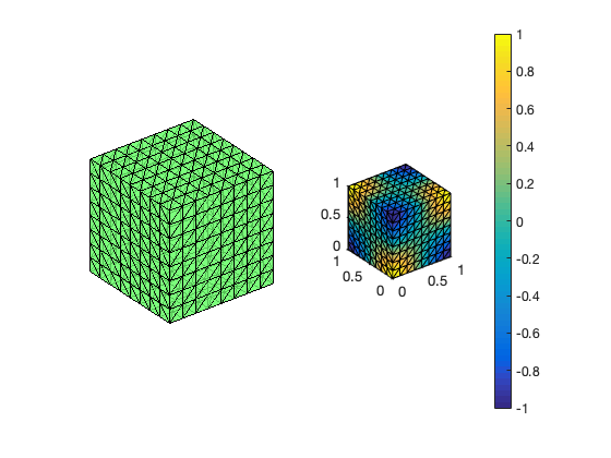
%% Setting
[node,elem] = cubemesh([0,1,0,1,0,1],1/3);
mesh = struct('node',node,'elem',elem);
option.maxIt = 4;
option.elemType = 'P2';
option.printlevel = 1;
option.plotflag = 1;
%% Non-empty Dirichlet boundary condition.
fprintf('Mixed boundary conditions. \n');
% pde = polydata3;
pde = sincosdata3;
mesh.bdFlag = setboundary3(node,elem,'Dirichlet','~(x==0)','Neumann','x==0');
femPoisson3(mesh,pde,option);
Mixed boundary conditions.

 Multigrid V-cycle Preconditioner with Conjugate Gradient Method
#dof:     3600,  #nnz:    70718, smoothing: (1,1), iter: 12,   err = 2.83e-09,   time = 0.13 s

 Multigrid V-cycle Preconditioner with Conjugate Gradient Method
#dof:    30752,  #nnz:   659134, smoothing: (1,1), iter: 12,   err = 3.80e-09,   time = 0.38 s

 Multigrid V-cycle Preconditioner with Conjugate Gradient Method
#dof:   254016,  #nnz:  5674430, smoothing: (1,1), iter: 12,   err = 3.57e-09,   time =  2.2 s
Table: Error
 #Dof        h        ||u-u_h||    ||Du-Du_h||   ||DuI-Du_h|| ||uI-u_h||_{max}

   729   2.500e-01   5.00700e-03   1.32387e-01   5.25032e-02   1.21275e-02
  4913   1.250e-01   6.03477e-04   3.52893e-02   9.25606e-03   1.61600e-03
 35937   6.250e-02   7.43413e-05   9.04712e-03   1.42917e-03   2.02649e-04
274625   3.125e-02   9.26851e-06   2.28115e-03   2.17441e-04   2.52582e-05

Table: CPU time
 #Dof    Assemble     Solve      Error      Mesh

   729   1.10e-01   2.00e-02   1.20e-01   1.00e-02
  4913   1.90e-01   1.30e-01   1.00e-01   1.00e-02
 35937   8.80e-01   3.80e-01   3.90e-01   7.00e-02
274625   6.22e+00   2.17e+00   3.01e+00   0.00e+00
Pure Neumann boundary condition
When pure Neumann boundary condition is posed, i.e., $-\Delta u =f$ in $\Omega$ and $\nabla u\cdot n=g_N$ on $\partial \Omega$, the data should be consisitent in the sense that $\int_{\Omega} f \, dx + \int_{\partial \Omega} g \, ds = 0$. The solution is unique up to a constant. A post-process is applied such that the constraint $\int_{\Omega}u_h dx = 0$ is imposed.
%% Pure Neumann boundary condition.
fprintf('Pure Neumann boundary condition. \n');
pde = sincosdata3Neumann;
option.plotflag = 0;
mesh.bdFlag = setboundary3(node,elem,'Neumann');
femPoisson3(mesh,pde,option);
Pure Neumann boundary condition.

 Multigrid V-cycle Preconditioner with Conjugate Gradient Method
#dof:      729,  #nnz:    13921, smoothing: (1,1), iter: 11,   err = 8.36e-09,   time = 0.06 s

 Multigrid V-cycle Preconditioner with Conjugate Gradient Method
#dof:     4913,  #nnz:   103105, smoothing: (1,1), iter: 12,   err = 3.57e-09,   time = 0.07 s

 Multigrid V-cycle Preconditioner with Conjugate Gradient Method
#dof:    35937,  #nnz:   792961, smoothing: (1,1), iter: 12,   err = 3.77e-09,   time = 0.35 s

 Multigrid V-cycle Preconditioner with Conjugate Gradient Method
#dof:   274625,  #nnz:  6218497, smoothing: (1,1), iter: 12,   err = 4.84e-09,   time =  2.2 s
Table: Error
 #Dof        h        ||u-u_h||    ||Du-Du_h||   ||DuI-Du_h|| ||uI-u_h||_{max}

   729   2.500e-01   4.33972e-03   1.06671e-01   1.11359e-01   2.69023e-02
  4913   1.250e-01   5.63932e-04   3.20352e-02   2.08121e-02   5.72678e-03
 35937   6.250e-02   7.20239e-05   8.63820e-03   3.68308e-03   8.55523e-04
274625   3.125e-02   9.12740e-06   2.22998e-03   6.44578e-04   1.14993e-04

Table: CPU time
 #Dof    Assemble     Solve      Error      Mesh

   729   1.00e-01   6.00e-02   4.00e-02   1.00e-02
  4913   1.60e-01   7.00e-02   9.00e-02   2.00e-02
 35937   8.10e-01   3.50e-01   4.20e-01   7.00e-02
274625   5.80e+00   2.21e+00   2.78e+00   0.00e+00
Robin boundary condition
%% Robin boundary condition.
fprintf('Robin boundary condition. \n');
pde = sincosRobindata3;
mesh.bdFlag = setboundary3(node,elem,'Robin');
femPoisson3(mesh,pde,option);
Robin boundary condition.

 Multigrid V-cycle Preconditioner with Conjugate Gradient Method
#dof:     4913,  #nnz:   105409, smoothing: (1,1), iter: 12,   err = 2.66e-09,   time = 0.05 s

 Multigrid V-cycle Preconditioner with Conjugate Gradient Method
#dof:    35937,  #nnz:   802177, smoothing: (1,1), iter: 12,   err = 4.68e-09,   time = 0.35 s

 Multigrid V-cycle Preconditioner with Conjugate Gradient Method
#dof:   274625,  #nnz:  6255361, smoothing: (1,1), iter: 12,   err = 8.75e-09,   time =  2.4 s
Table: Error
 #Dof        h        ||u-u_h||    ||Du-Du_h||   ||DuI-Du_h|| ||uI-u_h||_{max}

   729   2.500e-01   4.44278e-03   1.19113e-01   8.29341e-02   4.13848e-02
  4913   1.250e-01   5.66084e-04   3.35620e-02   1.48538e-02   3.95143e-03
 35937   6.250e-02   7.20911e-05   8.82519e-03   2.51203e-03   3.51203e-04
274625   3.125e-02   9.13225e-06   2.25306e-03   4.25087e-04   4.30278e-05

Table: CPU time
 #Dof    Assemble     Solve      Error      Mesh

   729   7.00e-02   1.00e-02   3.00e-02   0.00e+00
  4913   1.60e-01   5.00e-02   9.00e-02   2.00e-02
 35937   8.30e-01   3.50e-01   3.80e-01   7.00e-02
274625   6.04e+00   2.36e+00   2.94e+00   0.00e+00
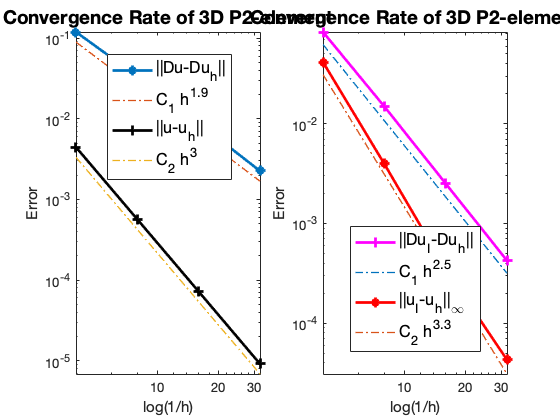
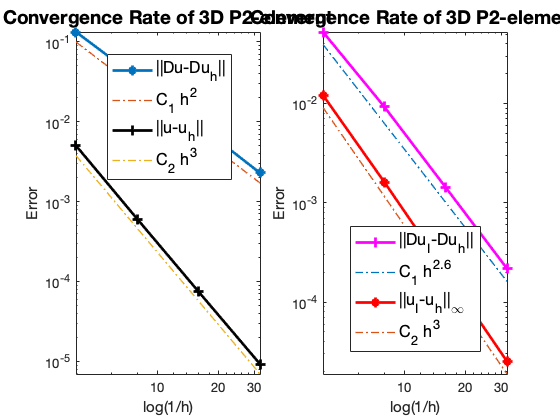
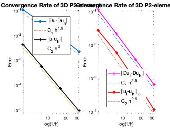
Conclusion
The optimal rate of convergence of the H1-norm (2nd order) and L2-norm (3rd order) is observed. Superconvergence between discrete functions $| \nabla u_I - \nabla u_h |$ is only 2.5 order.
For Neumann problem, the maximum norm is only 2.6 not optimal.
MGCG converges uniformly in all cases.
Comments