iFEM development notes

TODO

• Add the postprocessing to the domain with 1 cavity.
• Fix the code when there are two or more cavities.
• Currently the difference between $Qu - u_h$ can be used as an approximation to the harmonic field in that domain. Need to further verify this.
• prolongation and restriction operators in mgHodgeLapE.m is built for lowest order Nedelec elements.

mg

Warning: Matrix is close to singular or badly scaled. Results may be inaccurate. RCOND = 1.387779e-16.

In mg/vcycle (line 674)

When the matrix is singular, the coarse grid solver is changed to ‘pcg’ not ‘direct’.

if condest(Ai{1}) > 1e-12 % Ai{1} is singular
    coarsegridsolver = 'pcg';
end

coarsen3

• In the input and output, the ordering of arguments is changed to bdFlag, HB
• To use coarsen3 , HB is needed. Therefore add setup in label3 to initialize HB.

Version Changes

Functions in differenti versions of MATLAB might be different. To be compatible, use version check for unique function and DelaunayTri (earlier version) v.s. delaunayTriangulation (2014 and after).

Search matlabversion in iFEM folder to find all functions affected.

unique

In matlab, the behavior of unique has been changed. This includes:

  -	occurrence of indices in IA and IC switched from last to first
  -	IA and IC will always be column index vectors

If this change in behavior has adversely affected your code, you may 
preserve the previous behavior with:
  
     [C,IA,IC] = unique(A,'legacy')

In ifem, we need ‘last’. So in myunique function different call of unique is provided depending on the version of matlab.

Neumann problem

Previously I pitch one point and set u(1) = 0 , i.e. freeNode = 2:N and fixedNode =1. After that, enforce $\int_{\Omega} u = 0$ by a constant shift.

But this requires the exact solution satisfies the condition $u(x(1))=0$ which then fails for some data. In 2D, Poissonfemrate use sincosdata will give rate 1.8 while change to sincosNeuman will give optimal order 2.

In 3-D, the problem is worse. Rate 1.5 for Neuman and 1.3 for Robin for the error $|u_I - u_h|_{\infty}$ .

That’s reasonable. Solution to Neumann problem is not unique. We don’t know the constant and thus measured the maximum norm is not a well defined problem.

The question we should ask is:

is the solution we computed ONE solution of the system Au = f ?

So in the new formulation, I perturbe the matrix by A(1,1) = A(1,1) + 1e-6. Then the matrix is non-singular and use mg to solve the linear system.

The accuracy is still the same. No optimal order measured in the maximum norm.

One reason I suspect is the ill-conditioning of the sub-matrix. In 3-D, it is $h^{-3}$ while in 2D is $h^{-2}(1+

\log h

)$.

Reference

• P.B. Bochev, R.B. Lehoucq, On the Finite Element Solution of the Pure Neumann Problem, SIAM Rev. 47 (2005) 50–66.

My MG solver works pretty well but probably the ill-condition brings an issue to the perturbated problem.

The problem is still the same. We didn’t find a solution to $Au = b$ but a perturbated one. The perturbation is small in average (L2 type norm) but can be a problem for maximum problem.

Here is a simple perturbed analysis. We are solving $ (A + \epsilon) u_{\epsilon} = b$. Substract the equation $(A+\epsilon )u = b + \epsilon u$ to get the equation $ (A + \epsilon) e = \epsilon u$ and thus $|e|\leq | (A+\epsilon)^{-1}||\epsilon u|$. The matrix $A$ is singular and if $\epsilon < \lambda_2$, the norm $| (A+\epsilon)^{-1}| = \epsilon^{-1}$ and no control of the error. This is the stability issue due to the ill-conditioned matrix.

To solve the problem, we need to formulate a saddle point system to enforce the constaint $\int_{\Omega}u =0$ into the system which is not straight forward.

Conclusion Accept the current treatment and be aware that for pure Neumann problem, the rate of the computed solution in the maximum norm could be degenerated slightly especially in 3D.

Robin boundary condition in 3D

Again the maximum norm of the error is not optimal and the rate is only 1.3. Shuhao did some test and seems that the geometry of the domain will affect the maximum error. The following is revised from his email.

---

For first 2 tests, I used the same $\sin(x)\sin(y)\sin(z)$ as true solutions on $(0,\pi)^3$.

• Test 1: Only $x==0$ face as Robin boundary, and I hard-coded the nodeso n z-axis as Robin nodes, not fixed DoFs; optimal rate of converge for $L_{\infty}$ norm. The error concentrates on where $\Delta u$ is big.

  

  

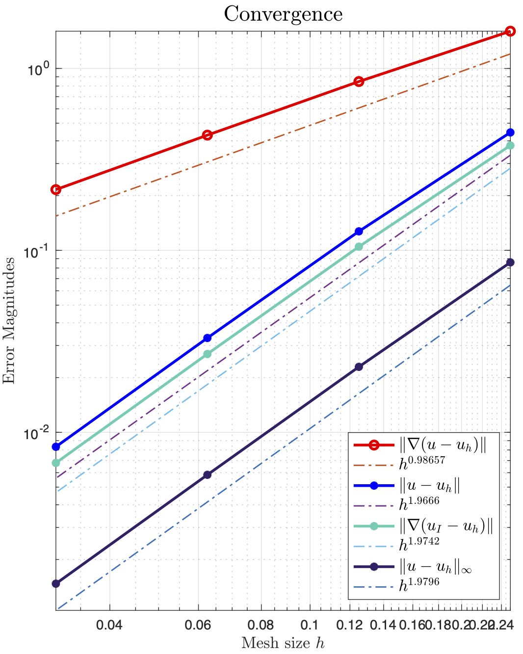
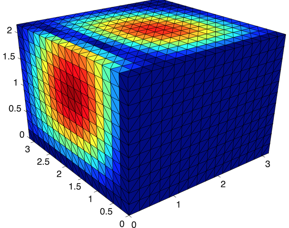
• Test 2: $x==0$ and $y==0$, as Robin boundary; suddenly the rate for $L_{\infty}$ becomes suboptimal, and the error concentrates on the edge where these two faces intersect.

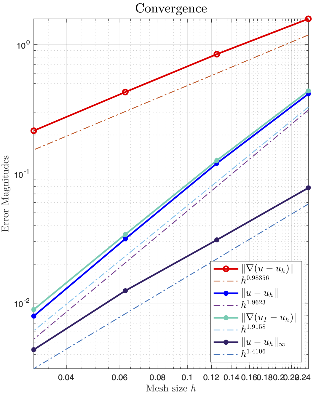
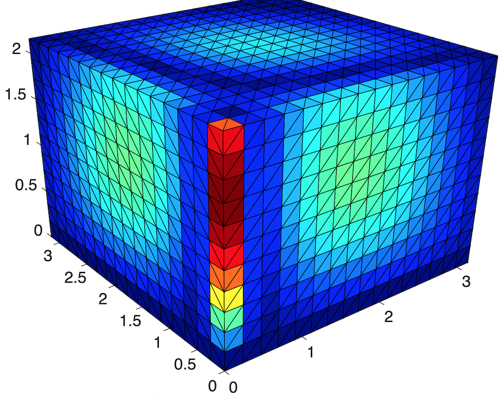
• Test 3: Now I suspected it is caused by geometry, so I used the distmesh in ifem to generate a ball-mesh problem. The L-inf becomes optimal again for pure Robin problem in $\Omega = {x^2+y^2+z^2 = 4}$, and the error is evenly distributed (maybe just for a few tetrahedra with bad mesh quality).

![

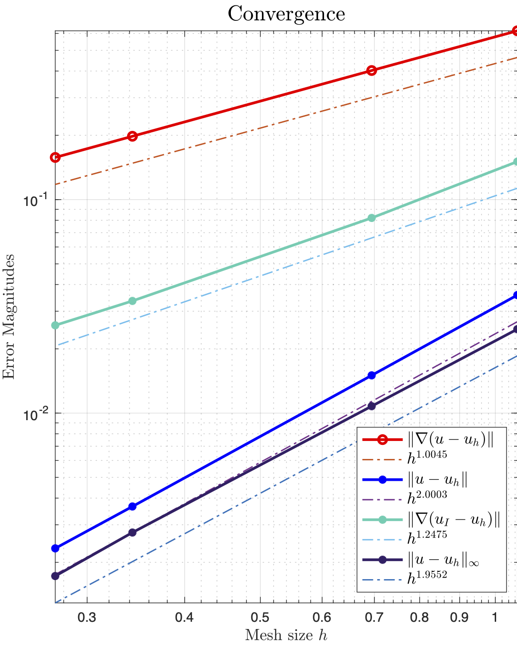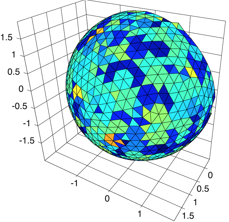
I think from the perspective of using Green function approach to prove $L_{\infty}$ estimate, locally $W_{2,\infty}$ is illy defined on cubes due to the exterior normal vectors is not continuous. In 2D, the problem is kinda minimal (you only have 4 points), so we still observe $h^2|\log(h)|$ rate of convergence.

In 2-D, the discrete Sobolev space embedding $|v_h|_{\infty}\lesssim (1+

\log h

)|\nabla v_h|$ implies the quasi-optimal rate.

---

Find a paper and will try later.

• M. Juntunen, R. Stenberg, Nitsche’s method for general boundary conditions, Math. Comp. 78 (2009) 1353–1374.

The boundary condition is \(\frac{\partial u}{\partial n}=\frac{1}{\epsilon}\left(u_{0}-u\right)+g \quad \text { on } \Gamma\) As $\epsilon \to \infty$, we obtain Neumann boundary condition and $\epsilon \to 0$ to get Dirichlet boundary condition.

The convergence is \(\left\|\nabla\left(u-u_{h}\right)\right\|_{L^{2}(\Omega)}+\epsilon^{-1 / 2}\left\|u-u_{h}\right\|_{L^{2}(\Gamma)} \leq C h^{s-1}\left(1+h_{\Gamma}^{1 / 2} \epsilon^{-1 / 2}\right)\|u\|_{H^{s}(\Omega)}\)

The condition number is \(\kappa=\mathcal{O}\left(h^{-2}+(\epsilon h)^{-1}\right)\)

FreeNode, FreeEdge, FreeDof

Change them to logical arrays. It might cause error when length(freeNode) is used.

mg

The input matrix could be

• AD + option.freeDof
• AD
• A(freeDof, freeDof) + option.freeDof

The AD is the whole matrix where the Dirichlet boundary condition is build-in by modifying the corresponding sub-matrix to an identity. So the size of AD can be used to determine several types of elements.

If only A(freeDof, freeDof) is given, we cann’t know the actual size of the original matrix. That information can be build into option.freeDof, which is a logical array. The size of option.freeDof will be used to determine several types of elements.

Multilevel Usage

femPoisson, femStokes are high level command.

Poisson, StokesP2P1, Maxwell etc are subroutines for different finite element and different equations.

squarePoisson, cubeMaxwell, squareStokes etc are middle level test functions.

So we need another level: int2d, int3d, int1d etc to compute the variational form for different elements. Then it can be used to do more equations.

Move some files to ifem_local

Some subroutines are not tested yet and thus move to ifem_local. Removed MaxwellH and Helmholtz for example.

Maxwell2 Neumann boundary condition

July 23, 2020

In the boundary surface integral, check the ordering

pidx = face(face2locEdge(s,1))< face(face2locEdge(s,2));
% phi_k = lambda_iDlambda_j - lambda_jDlambda_i;
% lambda_i is associated to the local index of the face [1 2 3]
% Dlambda_j is associtated to the index of tetrahedron
% - when the direction of the local edge s is consistent with the
%   global oritentation given in the triangulation, 
%           s(1) -- k(1),  s(2) -- k(2)
% - otherwise 
%           s(2) -- k(1),  s(1) -- k(2)
if pidx
    phi_k = lambda(pp,face2locEdge(s,1))*Dlambda(isBdElem,:,tetLocEdge(kk,2)) ...
lambda(pp,face2locEdge(s,2))*Dlambda(isBdElem,:,tetLocEdge(kk,1));
else
    phi_k = lambda(pp,face2locEdge(s,2))*Dlambda(isBdElem,:,tetLocEdge(kk,2)) ...
lambda(pp,face2locEdge(s,1))*Dlambda(isBdElem,:,tetLocEdge(kk,1));                   
end

But if all faces and edges are ascend ordering, then no need to check.

tetLocEdge = [1 2; 1 3; 1 4; 2 3; 2 4; 3 4]; % edge of a tetrahedral [1 2 3 4]
face2locEdge = [2 3; 1 3; 1 2]; % edge of the face [1 2 3]

Note that in face2locEdge, the second edge is [1 3] not [3 1]

And also make sure when call bdfaceintegral, the input face is ascend ordering.

    face = [2 3 4]; face2locdof = [6 5 4];
    if ~isempty(isBdElem)
        bdb = bdfaceintegral(isBdElem,face,face2locdof);

StokesBDM1bfemrate

July 24, 2020 11 - 12:49 PM

Spend 1.5 hour to correct a typo. Record the debug procedure.

1. The rate is not optimal and oscillation is observed. So it is wrong. Find backup 2019-06-05 which works well. So run two sessions and try to figure out the bug.
2. Change the solver to direct and make sure it is not caused by solvers.
3. Compare the final linear systems and found the matrix is different.
4. Put a breakpoint after several components of the big matrix is assembled and compare each component. Find the matrix R is different.
5. Check components involved in the assembling of R and found Meb from getmassmatvec is wrong.
6. diff two files and find the assembling is simplified. Copy back, then it works.
7. Then check more carefuly why the simplification is wrong and finally find a typo in the simplification

	+ DiDj(:,i1,i1)...
	+ DiDj(:,i1,i2));

line 151: the last line should be DiDj(:,i1,i2) but it must be copied from above line and still DiDj(:,i1,i1).

What is the lesson?

Test after any change.

Since BDM1B is used in StokesBDM1b, I should test when I change the code getmassmatvec . Then it will save the time to trace the bug.

Maxwell1saddle

The non-trivial part is to compute $\nabla p$ for $p\in P^2(\mathbb R^3)$. The grad matrix is for $P^1$ element which can be computed by the incidence matrix. For quadratic bubble functions, $4\lambda_i\lambda_j$ is map to $4\psi$. So in the hierachical basis, the matrix is a block diagonal \(\begin{pmatrix} {\rm grad} & 0 \\ 0 & 4 I \\ \end{pmatrix}.\) Pretty easy.

Now we need to express the quadratic nodal basis in terms of hierarchical basis. The nodal basis at vertex $i$ is $\eta_i = \lambda_i(2\lambda_i - 1)$. Express $\lambda_i = 1 - \sum_{j\neq i}\lambda_j$, we get \(\eta_i = 2\lambda_i(1 - \sum_{j\neq i}\lambda_j) - \lambda_i = \lambda_i - 2\sum_{j\neq i}\lambda_i\lambda_j.\) Then for the expansion in nodal basis \(\sum_i d_i \eta_i = \sum_i d_i\lambda_i - \sum_i 2d_i\left (\sum_{j\neq i}\lambda_i\lambda_j\right ).\) So there is a contribution from nodal to edge bubble. The grad matrix becomes \(\tag{G} \begin{pmatrix} {\rm grad} & 0 \\ e2v & 4 I \\ \end{pmatrix}.\)

Update Jul 30, 2020

Trying to fix the multigrid preconditioning for Maxwell1saddle.m.

Progress

• Mass matrix for $P^2$ element added.
• Fixed several discrepancies in setting up the auxiliaries matrices. The gradient matrix grad fed into mgMaxwell changed to bigGrad which is $(\rm G)$ above.

cubemesh

    shiftMatrix = [1 0 0; 0 1 0; -1/2 0 1/2]*...
                  [1 0 0; -1/2 1/2 0; 0 0 1]*...
                  [1 0 0; 0 1 0; 0 -1/2 1/2];
    nodeShift = node*shiftMatrix;
%     *[cos(pi/3), -sin(pi/3), 0; 1/2, 0, sqrt(3)/2; 1, 0, 0]);  
    % shift the square to a parallegram to select the diagonal in delaunay
    matlabversion = version();
    if str2double(matlabversion(end-5:end-2)) <= 2013
        T = DelaunayTri(nodeShift(:,1),nodeShift(:,2),nodeShift(:,3)); %#ok<*DDELTRI>
        elem = T.Triangulation;
    else
        T = delaunayTriangulation(nodeShift(:,1),nodeShift(:,2),nodeShift(:,3));
        elem = T.ConnectivityList;
    end
    elem = label3(node,elem);
    showmesh3(nodeShift,elem);

The Delaunay triangulation can’t pick the correct diagonal and thus it is different with the uniform grid. It will result different bisection.

Try to shift the cube to parallelpipe so that the diagonal can be consistent. But Delaunay is not robust and even shift the coplanar points to non coplanar and thus creates slivers.

Change the different length and different mesh size by loop over the index.

Primal-Dual Weak-Galerkin

Added a primal-dual weak-galerkin scheme in the /research folder.