Solvers for Poisson-type Equations
x = mg(A,b,elem) attempts to solve the system of linear equations Ax = b for x using geometric multigrid solvers. Inside mg, a coarsening algorithm is applied. The method is designed for the system from several finite element descritzations of elliptic equations on a grid whose topology is given by the array elem.
PDE
The classic formulation of the Poisson equation reads as
\[- \Delta u = f \text{ in } \Omega, \qquad u = g_D \text{ on } \Gamma _D, \qquad \nabla u\cdot n = g_N \text{ on } \Gamma _N,\]where $\partial \Omega = \Gamma _D\cup \Gamma _N$ and $\Gamma _D\cap \Gamma _N=\emptyset$. We assume $\Gamma _D$ is closed and $\Gamma _N$ open. The corresponding bilinear from \(a(u,v) := \int _{\Omega} \nabla u\cdot \nabla v\, {\rm dxdy}\) will lead to a symmetric and positive definite (SPD) matrix.
Variable diffusion coefficient is allowed, i.e. the operator $-\nabla \cdot( d \nabla u)$. When $d$ is highly oscillatory or anisotropic, the resulting SPD matrix is hard to solve.
Elements
x = mg(A,b,elem) works for linear finite element and mesh elem is obtained by uniformrefine, bisect, or uniformrefine3 by default. For other finite elements, more mesh structure, e.g., edge can be provided as varargin. If no extra input information, mg will try to guess the type of element by comparing the size of the system with the number of nodes and elements and construct needed data structure.
For 3-D adaptive grids obtained by bisect3, HB is needed for the coarsening, and should be listed as the first parameter in varargin. Interesting enough, for 2-D adaptive grids obtained by bisect, only elem is enough for the automatic coarsening. See coarsen.
Here is a list of possible elements.
- mg(A,b,elem)                      work in most scenario
- mg(A,b,elem,option,edge)          2-D quadratic P2 element or linear CR element
- mg(A,b,elem,option,HB)            3-D linear P1 element on adaptive meshes
- mg(A,b,elem,option,HB,edge)       3-D quadratic P2 element on adaptive meshes
- mg(A,b,elem,option,HB,face)       3-D non-conforming CR element on adaptive meshes
More input and output
x = mg(A,b,elem,options) specifies options in the following list.
- option.x0: the initial guess. Default setting x0 = 0.
- option.tol: the tolerance of the convergence. Default setting 1e-8.
- option.maxIt: the maximum number of iterations. Default setting 200.
- option.N0: the size of the coarest grid. Default setting 500.
- option.mu: smoothing steps. Default setting 1.
- option.coarsegridsolver: solver used in the coarest grid. Default
  setting: direct solver.
- option.freeDof: free d.o.f
- option.solver: various cycles and Krylov space methods
    * 'NO'     only setup the transfer matrix
    * 'Vcycle'      V-cycle MultiGrid Method
    * 'Wcycle'      W-cycle MultiGrid Method
    * 'Fcycle'      Full cycle Multigrid Method
    * 'cg'     mg-Preconditioned Conjugate Gradient
    * 'minres' mg-Preconditioned Minimal Residual Method
    * 'gmres'  mg-Preconditioned Generalized Minimal Residual Method
    * 'bicg'   mg-Preconditioned BiConjugate Gradient Method
    * 'bicgstable' mg-Preconditioned BiConjugate Gradient Stabilized Method
    * 'bicgstable1' mg-Preconditioned BiConjugate Gradient Stabilized Method
    The default setting is 'cg' which works well for SPD matrices. For
    non-symmetric matrices, try 'gmres' and for symmetric but indefinite
    matrices, try 'minres' or 'bicg' sequences.
    The string option.solver is not case sensitive.
- option.preconditioner:  multilevel preconditioners including:
    * 'V'   V-cycle MultiGrid used as a Preconditioner
    * 'W'   W-cycle MultiGrid used as a Preconditioner
    * 'F'   Full cycle Multigrid used as a Preconditioner
    * 'bpx' BPX-Preconditioner
- option.printlevel: the level of screen print out
    * 0: no output
    * 1: name of solver and convergence information (step, err, time)
    * 2: convergence history (err in each iteration step)
[x,info] = mg(A,b,elem) also returns information of the solver
- info.flag:
    * 0: mg converged to the desired tolerance tol within maxIt iterations
    * 1: mg iterated maxIt times but did not converge.
    * 2: direct solver
- info.itStep: the iteration number at which x was computed.
- info.time: the cpu time to get x
- info.err: the approximate relative error in the energy norm in err(:,1) and the relative residual norm(b-A*x)/norm(b) in err(:,2). If flag is 0, then max(err(end,:)) <= tol.
- info.stopErr: the error when iteration stops
Examples: Jump Coefficients
In Introduction to Fast Solvers, several examples has been presented for linear and quadratic elements. Here we present a harder example on a 3-D elliptic equation with jump coefficients. This documentation is based on example/solver/Poisson3jumpmgrate.m. Run this example to get more information.
\(-\nabla \cdot (\omega\nabla u) = f\quad \text{ in } \Omega=(-1,1)^3\) \(u = 1 \text{ on } x=1, \qquad u=0 \text{ on } x=-1\) \(\omega\nabla u \cdot n = 0\) on other boundary faces.
The diffusion coefficent $\omega$ is piecewise constant with large jump:
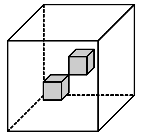
- $\omega(x) = 1$ if $x\in (-0.5, 0)^3$ or $x\in (0,0.5)^3$ and
- $\omega = \epsilon$ otherwise.
 }})
}})
Reference
Xu, J, and Y Zhu. “Uniform Convergent Multigrid Methods for Elliptic Problems with Strongly Discontinuous Coefficients.” M3AS 18, no. 1 (2008): 77–106.
%% Setting
% mesh
[node,elem,HB] = cubemesh([-1,1,-1,1,-1,1],1);
bdFlag = setboundary3(node,elem,'Dirichlet','(x==1) | (x==-1)');
mesh = struct('node',node,'elem',elem,'bdFlag',bdFlag);
% option
option.L0 = 3;
option.maxIt = 4;
option.elemType = 'P1';
option.printlevel = 1;
option.plotflag = 0;
option.dispflag = 0;
option.rateflag = 0;
% pde
pde = jumpmgdata2;
global epsilon
%% MGCG (multigrid preconditioned CG) solver
for k = 1:4
    epsilon = 10^(-k);
    [err,time,solver,eqn] = femPoisson3(mesh,pde,option);
    fprintf('\n Table: Solver MGCG for epislon = %0.2e \n',epsilon);
    colname = {'#Dof','Steps','Time','Error'};
    disptable(colname,solver.N,[],solver.itStep,'%2.0u',solver.time,'%4.2g',...
                      solver.stopErr,'%0.4e');
end
 Multigrid V-cycle Preconditioner with Conjugate Gradient Method
#dof:     4335,  #nnz:    28747, smoothing: (1,1), iter: 12,   err = 9.68e-09,   time = 0.09 s

 Multigrid V-cycle Preconditioner with Conjugate Gradient Method
#dof:    33759,  #nnz:   230043, smoothing: (1,1), iter: 13,   err = 2.68e-09,   time = 0.27 s

 Multigrid V-cycle Preconditioner with Conjugate Gradient Method
#dof:   266175,  #nnz:  1838395, smoothing: (1,1), iter: 13,   err = 3.23e-09,   time =  1.2 s

 Table: Solver MGCG for epislon = 1.00e-01
 #Dof   Steps Time      Error

  4913   12   0.09   9.6781e-09
 35937   13   0.27   2.6850e-09
274625   13    1.2   3.2292e-09


 Multigrid V-cycle Preconditioner with Conjugate Gradient Method
#dof:     4335,  #nnz:    28747, smoothing: (1,1), iter: 13,   err = 9.53e-09,   time = 0.03 s

 Multigrid V-cycle Preconditioner with Conjugate Gradient Method
#dof:    33759,  #nnz:   230043, smoothing: (1,1), iter: 14,   err = 7.08e-09,   time = 0.24 s

 Multigrid V-cycle Preconditioner with Conjugate Gradient Method
#dof:   266175,  #nnz:  1838395, smoothing: (1,1), iter: 15,   err = 3.78e-09,   time =  1.2 s

 Table: Solver MGCG for epislon = 1.00e-02
 #Dof   Steps Time      Error

  4913   13   0.03   9.5332e-09
 35937   14   0.24   7.0849e-09
274625   15    1.2   3.7846e-09


 Multigrid V-cycle Preconditioner with Conjugate Gradient Method
#dof:     4335,  #nnz:    28747, smoothing: (1,1), iter: 14,   err = 2.24e-09,   time = 0.03 s

 Multigrid V-cycle Preconditioner with Conjugate Gradient Method
#dof:    33759,  #nnz:   230043, smoothing: (1,1), iter: 15,   err = 3.29e-09,   time = 0.24 s

 Multigrid V-cycle Preconditioner with Conjugate Gradient Method
#dof:   266175,  #nnz:  1838395, smoothing: (1,1), iter: 16,   err = 4.03e-09,   time =  1.2 s

 Table: Solver MGCG for epislon = 1.00e-03
 #Dof   Steps Time      Error

  4913   14   0.03   2.2379e-09
 35937   15   0.24   3.2873e-09
274625   16    1.2   4.0262e-09


 Multigrid V-cycle Preconditioner with Conjugate Gradient Method
#dof:     4335,  #nnz:    28747, smoothing: (1,1), iter: 14,   err = 2.36e-09,   time = 0.02 s

 Multigrid V-cycle Preconditioner with Conjugate Gradient Method
#dof:    33759,  #nnz:   230043, smoothing: (1,1), iter: 15,   err = 5.82e-09,   time = 0.24 s

 Multigrid V-cycle Preconditioner with Conjugate Gradient Method
#dof:   266175,  #nnz:  1838395, smoothing: (1,1), iter: 17,   err = 4.51e-09,   time =  1.3 s

 Table: Solver MGCG for epislon = 1.00e-04
 #Dof   Steps Time      Error

  4913   14   0.02   2.3592e-09
 35937   15   0.24   5.8153e-09
274625   17    1.3   4.5142e-09
%% V-cycle solver
for k = 1:4
    epsilon = 10^(-k);
    option.mgoption.solver = 'Vcycle';
    [err,time,solver,eqn] = femPoisson3(mesh,pde,option);
    fprintf('\n Table: Solver V-cycle for epislon = %0.2e \n',epsilon);
    colname = {'#Dof','Steps','Time','Error'};
    disptable(colname,solver.N,[],solver.itStep,'%2.0u',solver.time,'%4.2g',...
                      solver.stopErr,'%0.4e');
end
Multigrid Vcycle Iteration
#dof:     4913,  #nnz:    28747, smoothing: (1,1), iter: 31,   err = 7.92e-09,   time = 0.14 s
Multigrid Vcycle Iteration
#dof:    35937,  #nnz:   230043, smoothing: (1,1), iter: 34,   err = 8.42e-09,   time = 0.33 s
Multigrid Vcycle Iteration
#dof:   274625,  #nnz:  1838395, smoothing: (1,1), iter: 35,   err = 8.12e-09,   time =  2.8 s

 Table: Solver V-cycle for epislon = 1.00e-01
 #Dof   Steps Time      Error

  4913   31   0.14   7.9248e-09
 35937   34   0.33   8.4179e-09
274625   35    2.8   8.1222e-09

Multigrid Vcycle Iteration
#dof:     4913,  #nnz:    28747, smoothing: (1,1), iter: 83,   err = 8.29e-09,   time = 0.09 s
Multigrid Vcycle Iteration
#dof:    35937,  #nnz:   230043, smoothing: (1,1), iter: 122,   err = 8.88e-09,   time = 0.92 s
Multigrid Vcycle Iteration
#dof:   274625,  #nnz:  1838395, smoothing: (1,1), iter: 151,   err = 9.18e-09,   time =  9.6 s

 Table: Solver V-cycle for epislon = 1.00e-02
 #Dof   Steps  Time      Error

  4913    83   0.09   8.2928e-09
 35937   122   0.92   8.8789e-09
274625   151    9.6   9.1830e-09

Multigrid Vcycle Iteration
#dof:     4913,  #nnz:    28747, smoothing: (1,1), iter: 122,   err = 9.89e-09,   time = 0.23 s
Multigrid Vcycle Iteration
#dof:    35937,  #nnz:   230043, smoothing: (1,1), iter: 200,   err = 2.44e-07,   time =  1.3 s
NOTE: the iterative method does not converge!
Multigrid Vcycle Iteration
#dof:   274625,  #nnz:  1838395, smoothing: (1,1), iter: 200,   err = 4.59e-05,   time =   12 s
NOTE: the iterative method does not converge!

 Table: Solver V-cycle for epislon = 1.00e-03
 #Dof   Steps  Time      Error

  4913   122   0.23   9.8922e-09
 35937   200    1.3   2.4413e-07
274625   200     12   4.5888e-05

Multigrid Vcycle Iteration
#dof:     4913,  #nnz:    28747, smoothing: (1,1), iter: 130,   err = 8.91e-09,   time = 0.37 s
Multigrid Vcycle Iteration
#dof:    35937,  #nnz:   230043, smoothing: (1,1), iter: 200,   err = 1.16e-06,   time =  1.3 s
NOTE: the iterative method does not converge!
Multigrid Vcycle Iteration
#dof:   274625,  #nnz:  1838395, smoothing: (1,1), iter: 200,   err = 2.17e-04,   time =   11 s
NOTE: the iterative method does not converge!

 Table: Solver V-cycle for epislon = 1.00e-04
 #Dof   Steps  Time      Error

  4913   130   0.37   8.9149e-09
 35937   200    1.3   1.1554e-06
274625   200     11   2.1676e-04
Conclusion
For 3-D jump coefficients problem, MGCG (multigrid preconditioned CG) solver converges uniformly both to the mesh size and the ratio of the jump.
V-cycle alone doesn’t converge for small epsilon and small h.
Comments